The Relationship Between Monetary Policy and Asset Prices: A New Approach Analyzing U.S. M&A Activity

III. A New Approach: Mergers and Acquisitions

To begin this section, I emphasize that M&A activity has not been studied in relation to the effects of monetary policy on asset prices.¹¹ The only two types of assets considered in the literature have been stock prices and housing prices, even though M&A transactions are ideal for several reasons. First,M&Aactivity involves the equity prices of companies, just as stock prices reflect the equity value of public companies.¹² It follows that, if stock prices are relevant to study the effects of monetary policy on asset prices, then M&A activity must be relevant as well because they both measure the same type of asset. However, M&A transactions involve a multi-month process. Contrary to only observing one-day movements in stock prices, M&Aprocesses have the time to absorb shocks in monetary policy and respond accordingly. This allows empirical research to more consistently observe the effects of shocks. Unlike investing in a house that covers multiple decades or the perpetuity nature of stock valuations, M&A investments often cover a three to seven year window. This is more likely to reflect the effect of monetary policy, which controls the shortterm nominal rate. In the very least, M&A activity is a relevant asset class due to its enormous market size. In 2012 alone, over 14,000 M&A transactions were completed with an average value above $200 million. This empirical analysis of the effects of monetary policy on M&A activity provides an original approach to this literature and helps further understand the relationship between asset prices and monetary policy.

M&A transactions are either the merger of or purchase of companies, generally involving the sale of a majority stake or the entirety of a company. Broadly speaking, M&A involves two classes of acquirers: 1) a company acquiring or merging with another company; or 2) an investment institution, primarily a private equity firm, that acquires companies to include in an investment portfolio. The latter sort of acquisitions often involve a large portion of debt with only a minority of the acquisition being funded with equity. To understand this process, consider a typical private equity firm. The firm will raise capital in an investment fund and then acquire a group of companies, financing the acquisitions with debt. Each portfolio company has two primary goals: 1) use the investment from the acquisition to grow the company; and 2) generate profits that are used to pay down the debt. As the companies grow and the debt paid down, the private equity firm re-sells each company hopefully at a higher price due to growth. What is more, the firm receives a quantity worth the entire value of the company, which is sizably more than the original investment that was financed only partially with equity and mostly with debt. Even if only some of the portfolio companies grow and not all the debt paid down, the portfolio can post remarkable returns. Harris et al. (2013) has found that the average U.S. private equity fund outperformed the S&P 500 by over 3% annually. The next sections discuss more fully the elements of this market.

Asymmetric information is especially of concern in the M&A market. As noted earlier, over 14,000 M&A transactions occurred in 2012. Although this is a large market due to the size of each transaction, the frequency of transactions pales in comparison, say, to the thousands of stocks traded daily. The market value of a stock is readily available because of the high frequency of transactions that signal the price to market participants. In contrast, there may only be a few transactions each year that are similar in terms of size, sector, maturity, geography, etc. This asymmetry is further compounded when considering reporting requirements. Public companies are required to publish quarterly and annual financial reports. What is more, these reports include sections of management discussion, providing deeper insight into the prospects and growth of the companies. However, because many M&A transactions deal with private companies, this information is often not available. For this very reason, investment banks are hired to advise M&A transactions, gather and present company information to potential buyers, and provide a credible reputation to stand behind the company information, thus removing the asymmetry problem. Posing even more of a challenge for empirical research such as this, not all M&A deals are required to disclose the transaction price or valuation multiples. Therefore, particularly when assessing the aggregate market, one must be prudent in selecting relevant variables that are still reliable and consistent despite this lack of information.

When analyzing aggregate data on M&A, four variables reflect the overall market activity: 1) the aggregate value of all disclosed deals, 2) the average size of each deal, 3) the number of deals in each period, and 4) the average valuation multiple of each deal. I argue that the first two are inconsistent metrics due to reporting requirements. Because information is only available on disclosed transactions, the aggregate value of all deals does not represent the entire market and can fluctuate from period to period simply if more or fewer firms disclose deal information. Similarly, the average size of each deal can also fluctuate from period to period as this average size comes from only the sample of deals that are disclosed. For these variables, there is the potential for inconsistency from one period to the next based only on fluctuations in reporting.

The next two variables, however, account for these issues. The total number of M&A transactions represents both disclosed and nondisclosed deals, thus removing the disclosure problem altogether. Looking at the final variable, valuation multiples are disclosed for only a portion of transactions. However, unlike the average deal size, multiples are independent of the size of a company and reflect the real price of the company. If a company with $100 million in revenue is sold for $200 million, the enterprise value (EV) to its revenue, or the revenue multiple, would be 2.0x.¹³ If a company with $1 billion in revenue is sold for $2 billion, the revenue multiple would still be 2.0x. Regardless of company size, the average multiple is not distorted. Several common multiples are a ratio of EV to revenue, EBIT (earnings before interest and taxes), and EBITDA (earnings before interest, taxes, depreciation, and amortization). Without digging deeply into the accounting for each multiple, this study looks at the EBITDA multiple which is the most commonly used multiple in the investment banking industry. EBITDA indicates a company's operational profitability. In other words, it reflects how much a company can earn with its present assets and operations on the products it manufactures or sells. This multiple is comparable across companies regardless of size, gross margin levels, debt-capital structures, or any one time costs that affect net income. EBITDA is generally considered the truest accounting metric for the health and profitability of a company. Thus, the EBITDA multiple is an excellent pricing metric to determine the value of a company relative both across time and to other companies of varying sizes. When assessing aggregate data, the average EBITDA multiple is a proxy for the average real price of transactions. With these metrics in mind, I now discuss common valuation methods.

Valuation methods can be broken into two main categories: 1) Relative methods that value the company in comparison to similar companies; and 2) Intrinsic methods that value the company based on its own performance. Two types of relative methods are precedent transactions and comparable public companies ("comps"). Precedent transactions look at the financial metrics of similar M&A deals and then apply those multiples and ratios to the target company. Similarly, comps analysis examines the trading multiples of a group of similar public companies and applies them to the financials of the company. In each method, the sample is based on criteria such as industry, financial metrics, geography, and maturity. An analysis will take the multiples of the group of companies, say the EBITDA multiple, and then apply it to the company at hand. As an example, if the average EBITDA multiple of the precedent transactions or comps is 10.0x and the EBITDA of the company is $20 million, the relative methods imply a value of $200 million.

In addition to relative methods, intrinsic methods value a company based solely on its individual financials. Discounted cash flow ("DCF") analysis is the present value of a company's future cash flow, as the real worth of a company is determined by how much cash (income) it can generate in the future. This mirrors the basic asset price valuations discussed previously. A DCF is usually split into two parts. The first component of a DCF is the forecast of a company's free cash flow over a five to ten year period that is then divided by a discount rate to yield a present value. The most commonly used discount rate is the WACC which is broken into components based on a firm's capital structure. Debt and preferred stock are easy to calculate as they are based on the interest rate of debt or the effective yield of preferred stock. The cost of equity is determined using the Capital Asset Pricing Model ("CAPM") by taking the risk-free rate, i safe, and adding the product of the market risk premium, φ, and a company-specific risk-factor, β.¹⁴ Within the CAPM, the risk-free rate is often a 10-year Treasury bond whereas the market risk premium is generally the percentage that stocks are expected to outperform the riskless rate. The CAPM is given by Equation 7:

The three components must be added back together to determine one discount rate, usually calculated by theWeighted Average Cost of Capital ("WACC"). Depicted in Equation 8 below, WACC multiplies each cost by that component's percentage of the total capital structure.

The last part of the DCF is a terminal value to reflect the earnings of the company that are generated beyond the projection period. The Gordon Growth Method, a common terminal value, takes the final year of projected free cash flow, multiplied by a projected annual growth rate of the company and then divided by the difference between the discount rate and the growth rate.¹⁵ Adding the discounted free cash flows and the terminal value, the total DCF with a five-year projection period is the following:

The DCF, although one of the most common valuation methods, is highly sensitive to assumptions, particularly for the projected growth of the company, the beta risk-factor, and the terminal value. This creates asymmetric information where the seller will inevitably have more information than the buyer. Adverse selection may even arise where all sellers, whether performing well or not, will present favorable assumptions as buyers do not have the same insight to whether or not such projections are realistic and probable. For this reason, transactions rely on the credibility of investment banks and the use of multiple valuation methods to minimize asymmetric information.

Another intrinsic method is the leveraged buyout model ("LBO"), a more advanced valuation method that is relevant to acquisitions that involve a large amount of debt such as private equity acquisitions. An LBO works for three key reasons:

1. Up-front cash payment on the part of the acquirer is reduced by issuing debt;
2. The cash flows generated by the company can be used to pay down the debt;
3. The return on the future re-sale totals the initial funds spent, the amount of debt paid down, and any additional value from the company's growth.¹⁶

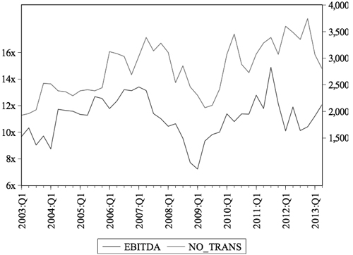
Briefly, I illustrate these three points in an example. Consider a private equity firm that acquires a $300 million portfolio company with $100 million of its own equity and finances the rest of the acquisition by issuing $200 million in debt. Over the course of several years, the investment in the company allows it to grow while also using its profits to pay down the $200 million in debt. Then, the private equity firm can re-sell the company at a higher price, earning a substantial return on the original equity investment. Although highly stylized, this illustrates how the more advanced LBO can yield above-market returns, as found in the Harris et al. study.

By applying the Asset Price Channel from the previous section to M&A activity, the potential effects of monetary policy are very similar to those of stock prices. For simplicity, let's only look at the DCF as an example. If the Fed raises the interest rate, the DCF could lower for several reasons. This could increase the interest rate on debt and i^safe17 What is more, this increase in the interest rates may discourage borrowing by the firm to fund additional investment projects. As a result, the projected annual growth in cash flows may decrease. In addition to these two issues, the WACC may be affected as well. The monetary policy shock is likely to make output more volatile, including the risk of the entire market and the firm, causing β to increase. A higher β results in a higher WACC. All of these components would result in a lower valuation of a firm. This DCF analysis illustrates the Asset Price Channel. If this theory holds, then one would expect the data to show that an increase in the interest rate by the Fed leads to a decrease in the number of M&A transactions and in the average EBITDA multiple.

IV. Data

The data considered in this study is broken into three groups: 1) M&A metrics, 2) interest rates, and 3) Taylor rule variables. The M&A data was made available by Dealogic, a research firm that specializes in providing information to investment banks and brokerage firms. The data gathered by Dealogic covers over 99% of all M&A activity across the globe. This dataset includes quarterly data from 2003 through 2013 on the total number of transactions in each period, the total value of all disclosed transactions, the average deal value of disclosed transactions, and average EBITDA multiple of disclosed transactions.¹⁸

As discussed in the previous M&A sections, the analysis below does not include the total value of all disclosed transactions or the average deal value of disclosed transactions because of inconsistencies in the sample of what deals are disclosed from one period to the next. Therefore, I focus on the number of total transactions which represents disclosed and non-disclosed deals and the average EBITDA multiple which is consistent regardless of sampling. Over this time period, the average EBITDA multiple was 11.12x and the average number of transactions per quarter was 2,793.

Below, Figure 1 displays the quarterly data for average EBITDA and number of transactions from 2003:Q1 to 2013:Q2. First, notice the steep decline in both price and activity in 2008 and 2009 as the financial crisis created great uncertainty and panic in the M&A market, causing investment activity to stagnate. A rebound followed that eventually led to record highs in number of transactions in 2011 and 2012. Also, this time series illustration shows the close relationship between these variables. Like any market, when the demand goes up and the quantity of transactions increases, this is accompanied by an increase in price. The M&A market is no different as the number of transactions and the average EBITDA multiple trend together.

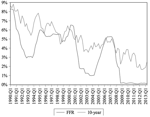
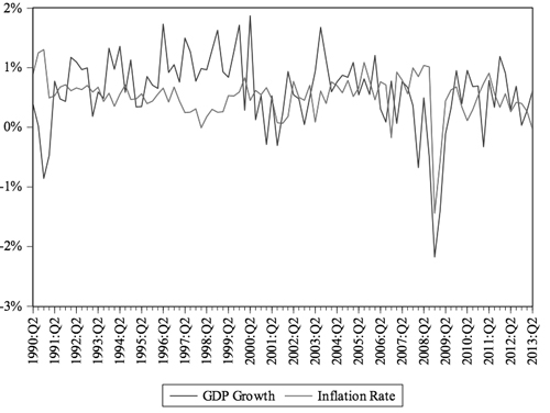
The remaining variables were gathered from the Federal Reserve Economic Data ("FRED"). In selecting an interest rate, the choice consistent with previous empirical studies is the federal funds rate ("FFR"). As discussed previously, the FFR is subject to a zero lower bound which was reached in 2009. The data on this will depict inaccurate results from 2009 to 2013 because the linear model would no longer hold. Thus, the dataset is cut-off in 2008. Because of this limited timeframe, this empirical study also includes the ten-year Treasury rate. As the study will show later, this still provides a consistent depiction of monetary policy transmission when modeling the Taylor rule. Because the ten-year rate never reaches its zero lower bound, this second interest rate allows the empirical analysis to consider the full MA dataset from 2003 through 2013. What is more, much of recent monetary policy actions have aimed to also affect long-term interest rates. Even from a monetary policy perspective beyond logistics with the data, the ten-year rate is natural to include in this analysis alongside the FFR.

For both the FFR and the ten-year, the end of period values are used, implying that the Federal Reserve responds to the macroeconomic variables in that current period whereas a change in the interest rate is likely to have a delayed effect on the macroeconomic variables. Thus, although the end of period is used for the interest rates, the average of the quarterly period is used for the Taylor rule variables. Finally, in order to analyze alongside the following Taylor rule variables, the data for both interest rates begin in 1990 with the FFR ending in 2008 and the ten-year ending in 2013. From 1990 through 2008, the average FFR was 4.23%. From 1990 through 2013, the average ten-year rate was 5.05%. Figure 2 highlights several key points concerning the FFR and the ten-year rates. First, this shows the ZLB that the FFR reached in late 2008, a bound that it has stayed at through 2013.

Secondly, this time series graph illustrates that the ten-year rate is a good proxy for the FFR as the two interest rates move together, reaching peaks and troughs at roughly the same time periods. The FFR moves more extremely, yet more smoothly than the ten-year rate. Because it is controlled by the Fed, the FFR changes in a disciplined, gradual manner whereas the ten-year rate faces more frequent fluctuations due to other market forces. However, the FFR also moves more extremely, particularly for cuts in the FFR. This is evident from 1992 to 1993, 2001 to 2004, and from 2008 to the present. In each case, the Fed cut rates aggressively in efforts to adequately respond to a slumping economy. Even though the ten-year rate decreases during these periods, the troughs are less severe.¹⁹

The final group of variables are the Taylor rule parameters which includes real GDP and inflation. The metric for GDP is the seasonally adjusted, quarterly average of the natural log of billions of chained 2009 dollars. Similarly, inflation is measured by the quarterly average of the natural log of the seasonally adjusted personal consumption index. The inflation rate is simply the difference of these natural logs. Again, the data for both variables is quarterly from 1990 through 2013. The average log of GDP and of the price level during this time period was 9.4 and 4.5, respectively. Figure 3 displays the difference of natural log for GDP and of the price level from 1990 to 2013.²⁰

Inflation has been remarkably stable over this time period, remaining steady around 0.5% per quarterly, or roughly 2% annually. This reflects the Fed's success in maintaining its target inflation rate. The one noticeable exception is the sharp deflation of 1.4% in 2008:Q4, which was in the heart of the Great Recession. Secondly, the late 1990s saw steady GDP growth as the quarterly growth rate increases significantly from 1996 through 2000. This line also shows the true impact of the Great Recession on the economy where GDP growth decreases severely and is negative for most of 2007 to 2010.

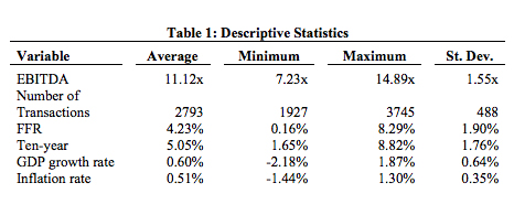
Below is a table of all the descriptive statistics of all the variables. EBITDA is presented as a multiple representing the total value of the transaction divided by the EBITDA. Also, the minimum of the FFR is 0.16%, which occurs in 2008, signaling the ZLB. Finally, as mentioned above, both GDP and inflation are reported as the differences of natural logs, which is the quarterly growth rate. The levels of GDP and PCE are not of importance, but only the natural logs which reflect the GDP growth rate and the inflation rate. In the actual model, the natural log is used rather than the difference in natural logs.

V. Method

A vector autoregression ("VAR") is an estimation technique that captures linear interdependence among multiple time series by including the lags of variables. In such a model, each variable has its own equation that includes its own lags and the lags of other variables in a model. Together, the entire VAR model has simultaneous equations that provide a model for how variables affect each other intertemporally. Bernanke and Mihov (1998) famously argue that such VARbased methods can be applied to monetary policy because VAR innovations to the FFR can be interpreted as innovations in the Fed's policy. Thus, a VAR model can be created using the current FFR and its lags alongside the current and lagged values of other macroeconomic variables. This allows empirical analysis to then determine the effects of innovations in monetary policy on other variables. In this study, because the M&A data overlaps the monetary interest rates, GDP, and inflation for a limited sample, I am using a modified VAR technique. Think of this model as establishing a Taylor rule using inflation and real GDP. The residuals in this equation are exogenous monetary shocks, that is, deviations from the Taylor rule. A second step then inputs these shocks – the residuals – into another VAR with the MA data.

In the results below, I include a VAR of the FFR and the ten-year rate with the Taylor rule variables. This illustrates the basics of the VAR technique and the intertemporal relationships between monetary policy innovations and macroeconomic variables. It is also important to include a word on the ordering of variables. By including the interest rate last, it suggests that monetary policy responds immediately to the current levels of GDP and inflation whereas the effects of the current interest rate really only have lagged effects on the macroeconomy.²² When ordering a VAR, an implicit assumption is being made about the timing of the intertemporal responses. Together, Equations 10-12 create a VAR model portraying a form of the Taylor rule

In an ideal case, one would run the same VAR above while including a fourth variable that measures MA activity. However, given the limited data set with the ZLB, I employ the two-step VAR technique described above to assess the effects of monetary policy shocks on MA activity. Using Equations 10-12 for both the FFR and the tenyear Treasury rate, I find the fitted values for the interest rate given the parameters of the model. The residuals of the interest rates from the VAR model can then be calculated using Equation 13 where i is the actual value of the interest rate, i^{^} is the estimated value of the interest rate, and e_i is the residual.

The residuals reflect monetary policy that differs from the Taylor rule, or shocks to monetary policy. By using this historical data in this way, the model extracts exogenous shocks in monetary policy for the period covering the M&A data.

The next step in this technique is to take these residuals and create another VAR model, this time using the current and lagged values of the residual shocks and the M&A data.²³ This model is given by Equation 14:

This VAR model will then allow for the same sort of impulse response functions that were discussed previously for illustrating the Taylor rule. However, in this case, the impulse is an actual change in the residual, or monetary policy shock. If the Asset Price Channel holds, M&A activity will decrease when the interest rate increases. Thus, a positive impulse to the residual would cause the average EBITDA multiple and the number of transactions to decrease.Continued on Next Page »