|
From The Developing Economist VOL. 1 NO. 1 The Relationship Between Monetary Policy and Asset Prices: A New Approach Analyzing U.S. M&A Activity
By Brett R. Ubl
The Developing Economist
2014, Vol. 1 No. 1 | pg. 3/3 | «
From Equations 10-12 the first VARs presented are linear, inertial Taylor rules using the lagged and contemporaneous values of the interest rate, GDP, and the price level.24 The first and primary purpose of this VAR is to take the residuals between the fitted FFR values and the actual FFR values. Applying Equation 13, this creates the exogenous shocks, or innovations, in the FFR that cannot be explained by the model. Over the period from 2003 to 2008, these residuals serve as the monetary policy shocks that will be used to analyze M&A activity. This VAR has an F-statistic of 120.35 and an R-squared value is 0.967. Next, I repeat this process using the 10-year rate in a VAR alongside GDP and inflation. In this VAR, the R-square is even stronger with a value of 0.999, and the F-statistic is 8102.57. The residuals are thus statistically significant and can be used as proxies for exogenous innovations in monetary policy.
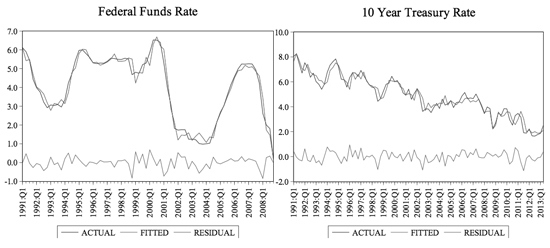
Figure 5: Actual Interest Rate vs. Taylor-Rule Estimation
Another way to confirm the validity of this VAR Taylor rule is to compare the actual interest rate values to the fitted values from the VARs. As Figure 5 illustrates, the fitted values mirror the actual values very closely. The difference between the actual and fitted values are movements in the interest rate where the Fed is not responding to output and inflation, representing shocks that can be placed into a second VAR with the M&A data.
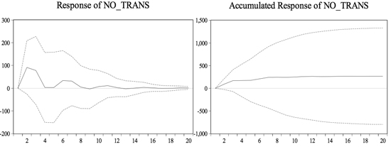
Equation 14 is modeled with the number of transactions responding to the FFR shocks, or residuals from the above graphs. The Rsquared is 0.67 with an F-statistic of only 2.74. This is in larger part due to the limited data range from 2003 to 2008 that is further restricted by the inclusion of lagged values. Figure 5 illustrates the simulation of a shock of one standard deviation to the FFR residual in this VAR model on the number of transactions. This simulates a roughly exogenous 30 basis-point increase in the FFR. The response of the number of transactions has an initial positive increase of roughly fifty to two hundred transaction per quarter. The accumulated response levels off at roughly 575 transactions after six quarters. Multiplying the quarterly average by six, this number of transactions is a 3.4% increase in the number of transactions. This is in the direction opposite of what would be predicted by the Asset Price Channel. Most importantly, the standard error bands in the graph indicate that the response is not statistically significant.25 This not only provides evidence against the Asset Price Channel, but it also contradicts the hypothesis.
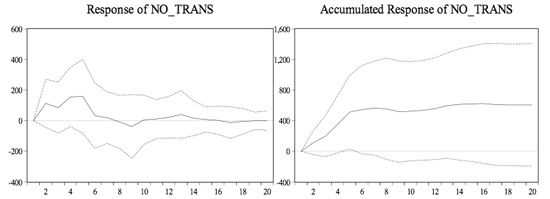
Figure 6: Response of Number of Transactions to a One S.D. Shock in the FFR Residual ±2S.E.
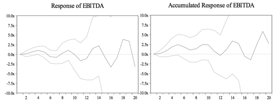
This process is repeated using the FFR residuals and EBITDA. The R-squared is 0.67 with an F-statistic of 2.82. As Figure 7 highlights, the EBTIDA response to a simulated one standard deviation shock to the FFR residual is not statistically significant. Only a limited portion of this projection period is relevant. For example, in quarter 14, the accumulated response is roughly 4x which is not even a realistic response given that the average EBITDA is only 11x. This suggests that this particular model may not be reflecting the relationship correctly. Again, I stress that this is in large part be due to the limited data as this only covers 2003 to 2008 before the FFR reached the zero lower bound. Over the course of the first three years, the accumulated response of EBITDA fluctuates between 1 and 3x. 2x is roughly 20% of the average EBITDA so the magnitude of the response is considerable given the shock to the FFR is only 40 basis-points. Given the volatility of both EBITDA, the standard error bands confirm that this is not a statistically significant impulse response. It remains that there is no evidence to support the Asset Price Channel and actually limited evidence to contradict the explanation.
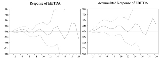
Figure 7: Response of EBITDA to a One S.D. Shock in the FFR Residual ±2S.E.
The above two VAR models are replicated using the residuals of the ten-year rate with an approximate 40 basis-points shock. Beginning with the number of transactions, this VAR has an R-squared of 0.60 with a stronger F-statistic of 5.4. The response of the number of transactions is not statistically significant, but is again positive. Looking at the accumulated response in Figure 8, the response flattens out around two hundred transactions by the end of the first projected year, or roughly 2% annually. A continuing theme exists in this VAR setup with no evidence supporting the Asset Price Channel and even slight evidence contradicting it.
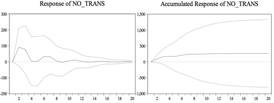
Figure 8: Response of Number of Transactions to a One S.D. Shock in the 10-year Rate Residual ±2S.E.
The final VAR model repeats the process using EBITDA with the residuals of the ten-year rate. This time, the R-squared is only 0.48 with an F-statistic of 3.34. Figure 9 illustrates the accumulated response of EBITDA to an approximate 40 basis-points shock to the tenyear rate residual. The response does not statistically differ from zero and peaks at 0.4x, or roughly 3.5%, in the second projected year. Like the other VAR models, this model provides no evidence in support of the Asset Price Channel and limited evidence against it.
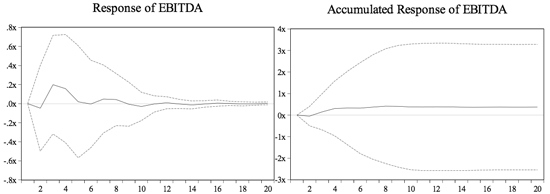
Figure 9: Response of EBITDA to a One S.D. Shock in the 10-year Rate Residual ±2S.E.
An alternative explanation places GDP as the primary driver of movements in asset prices. I hypothesize that the main concern of both investors and bankers is inevitably output – the production of the firm, of its industry, and of the entire economy. Thus, a positive shock to GDP should result in increases inM&Aprices and activity. By extracting the GDP residuals, exogenous shocks to GDP are identified that can then be modeled with the M&A data to determine the effect of output on M&A activity. I repeat the previous process by running Equations 10-14 using GDP, inflation, and the ten-year rate.26 This time, Equations 13 and 14 take the residuals of GDP to identify GDP shocks that are then modeled in a VAR with the M&A metrics.
In the VAR with GDP residuals and the number of transactions, a 0.6% quarterly shock to GDP has a statistically significant shock on the number of transactions. The accumulated response reaches a level around 900 transactions, or roughly 8% of the annual average number of transactions. This is strong evidence that GDP explains movements in M&A activity.
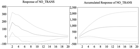
Figure 10: Response of Number of Transactions to a One S.D. Shock in the GDP Residual ±2S.E.
In the VAR with GDP residuals and the EBITDA multiple, a shock to GDP again leads to a positive response in the M&A metric. The GDP shock is approximately 0.5%. Despite being statistically insignificant, the magnitude of the shock reaches 1.4x, or roughly 12.5% of the average EBITDA multiple. This impulse response function is additional evidence supporting the explanation that GDP is a fundamental driver of movements in M&A activity.

Figure 11: Response of EBITDA to a One S.D. Shock in the GDP Residual ±2S.E.
When considering this alternative explanation, there is strong evidence in support of GDP as the primary explanation for movements in M&A prices and activity. A shock to GDP produces positive responses in both EBITDA and the number of transactions. I conclude that output is ultimately the primary driver of movements in the asset prices of M&A transactions. This is not a surprising result. At its fundamental level, the output of the firm, its industry, and the broader market drives M&A prices. Despite the persuasiveness of the Asset Price Channel, the data does not support this theory, but instead presents a simpler picture of movements in asset prices dependent solely on output.
This empirical study is an important addition to the monetary policy literature by considering a new asset class in M&A activity. Unlike the studies analyzing monetary policy with stock prices and housing prices, the Asset Price Channel does not hold with the number of M&A transactions and the average EBITDA multiple, reflecting both M&A activity and prices. Rather, the critical component in explaining movements in M&A activity is output. Although this empirical study does not find evidence of a relationship with monetary policy, it is still conceivable that an implicit relationship exists between monetary policy influencing output which then influences the M&A market. Regardless, this article does not find any direct relationship between monetary policy and M&A activity and therefore concludes that the Asset Price Channel does not hold. This study, then, is an important expansion of the literature and provides further understanding of the relationship between monetary policy and asset prices in the M&A market.
- Ball, Laurence M. 2012. Money, Banking, and Financial Markets. New York: Worth Publishers.
- Bernanke, Ben and Ilian Mihov. 1995. "Measuring Monetary Policy." Quarterly Journal of Economics. 113.3: 869-902.
- Bernanke, Ben and Kenneth Kuttner. 2005. "What Explains the Stock Market's Reaction to Federal Reserve Policy?" The Journal of Finance. 60.3: 1221-1257.
- Bernanke, Ben and Mark Gertler. 2001. "Should Central Banks Respond to Movements in Asset Prices?" The American Economic Review. 91.2: 253-257.
- Bernanke, Ben. 2010. "Monetary Policy and the Housing Bubble." Presented at the Annual Meeting of the American Economic Association. Board of Governors of the Federal Reserve System. Atlanta, Georgia, January 3.
- Bernanke, Ben. 2002. "On Milton Friedman's Ninetieth Birthday." Presented at the Conference to Honor Milton Friedman. University of Chicago. Chicago, Illinois, November 8.
- Bohl, Martin, Pierre Siklos, and Thomas Werner. 2007. "Do central banks react to the stock market? The case of the Bundesbank." Journal of Banking and Finance. 31.2:719-733.
- Bordo, Michael and Olivier Jeanne. 2002. "Monetary Policy and Asset Prices: Does ‘Benign Neglect' Make Sense?" International Finance. 5.2: 139-164.
- Bullard, James. 2013. "An Update on the Tapering Debate." Federal Reserve Bank of St. Louis, August 15.
- Bullard, James. 2007. "Seven faces of" the peril." Federal Reserve Bank of St. Louis Review. 339-352.
- Carlstrom, Charles and Timothy Fuerst. 2007. "Asset Prices, Nominal Rigidities, and Monetary Policy." Review of Economic Dynamics. 10: 256-275.
- Carlstrom, Charles and Timothy Fuerst. 2012. "Gaps versus Growth Rates in the Taylor rule." Federal Reserve Bank of Cleveland, October.
- Cecchetti, Stephen, et al. 2000. "Asset prices and Central Bank Policy." Paper presented at The Geneva Report on the World Economy No. 2. Geneva, Switzerland, May.
- Davig, Troy and Eric Leeper. 2007. "Generalizing the Taylor Principle." The American Economic Review. 97.3: 607-635.
- "DCF Questions Answers." 2012. Breaking Into Wall Street: Investment Banking Interview Guide.
- "Equity Value and Enterprise Value Questions Answers." 2012. Breaking Into Wall Street: Investment Banking Interview Guide.
- Erler, Alexander, Christian Drescher, and Damir Krizanac. 2013. "The Fed's TRAP: A Taylor-Type Rule with Asset Prices." Journal of Economics and Finance. 37.1: 136-149.
- Filardo, Andrew. 2000. "Monetary Policy and Asset Prices." Economic Review – Federal Reserve Bank of Kansas City. 85.3: 11-38.
- Gilchrist, Simon and John Leahy. 2002. "Monetary Policy and Asset Prices." Journal of Monetary Economics. 49.1: 75-97.
- Goodhart, Charles and Boris Hofmann. 2000. "Asset Prices and the Conduct of Monetary Policy." Presented at Sveriges Riksbank and Stockholm School of Economics Conference on Asset Markets and Monetary Policy. Stockholm, Sweden, June.
- Harris, Robert, et al. 2013. "Private Equity Performance: What do we know?" National Bureau of Economic Research. Forthcoming in Journal of Finance.
- Henderson, Nell. 2005. "Bernanke: There's No Housing Bubble to Bust." Washington Post, October 27.
- Iacoviello, Matteo. 2005. "House Prices, Borrowing Constraints, and Monetary Policy in the Business Cycle." The American Economic Review. 95.3: 739-764.
- Ida, Daisuke. 2011. "Monetary Policy and Asset Prices in an Open Economy." North American Journal of Economics and Finance. 22.2: 102-117.
- Laeven, Luc and Hui Tong. 2012. "US Monetary Shocks and Global Stock Prices." Journal of Financial Intermediation. 21.3: 530547.
- "LBO Model Questions Answers." 2012. Breaking IntoWall Street: Investment Banking Interview Guide.
- Rigobon, Roberto and Brian Sack. 2003. "Measuring the Reaction of Monetary Policy to the Stock Market." The Quarterly Journal of Economics. 118.2: 639-669.
- Rigobon, Roberto and Brian Sack 2004. "The Impact of Monetary Policy on Asset Prices." Journal of Monetary Economics. 51.8: 15531575.
- Taylor, John. 2007. "Housing and Monetary Policy." Federal Reserve Bank of Kansas City. 463-476.
- Taylor, John. 1993. "Discretion versus Policy Rules in Practice." Carnegie-Rochester Conference Series on Public Policy. 39: 195-214.
- "Valuation Questions Answers." 2012. Breaking Into Wall Street: Investment Banking Interview Guide.
- Wongswan, Jon. 2009. "The Response of Global Equity Indexes to U.S. Monetary Policy Announcements." Journal of International Money and Finance. 28.2: 344-365.
- I would like to recognize several individuals who enabled me to complete this project. First, I wish to extend appreciation to Agata Rakowski and Dealogic who provided the data on U.S. M&A activity. Also, my professional experience as an investment banking analyst with Robert W. Baird & Co. developed my understanding of the M&A market. I am thankful for the constant support of the University of Notre Dame's Department of Economics, especially Professors Michael Mogavero and Mary Flannery. Finally, I owe a heartfelt thanks to Professor Timothy Fuerst. His comments and whistling were an invaluable resource in this process. Indeed, I am forever grateful for the opportunity to learn under the Whistling Professor.
- By using Google Scholar and the University of Notre Dame's OneSearch for academic literature, I was unable to find any articles directly addressing M&A and monetary policy.
- The cases include the 1929 stock market crash, the 1980s housing and equity bubble in Tokyo, and the late 1990s crises in Southeast Asian equity and currency markets
- To clarify, the authors do not recommend that central banks should burst bubbles once they form as this could still lead to disastrous outcomes. Rather, they advocate for monetary policy that works to prevent bubbles from forming in the first place.
- This study diverges slightly from other analyses in that they consider optimal policy not only for busts but also more moderate asset price reversals following booms.
- This is the same critique that Cecchetti et al. considered, but then dismissed.
- As many of the critics have noted, identifying bubbles is no easy task. Recall that, even as late as 2005, Bernanke and the majority of central bankers did not realize the existence or extent of the housing bubble.
- It is generally assumed that the current inflation target of the Fed is approximately 2%.
- It is generally assumed that the current inflation target of the Fed is approximately 2%.
- Recall the Fisher Equation where the real rate is the difference between the nominal rate and the inflation rate. Thus, to move the real rate, the nominal rate needs to move by a larger amount than the inflation rate movement.
- The outline of the MA market and valuation methods follows the M&A investment banking guides by Breaking into Wall Street. ("Equity Value and Enterprise Value Questions Answers" 2012, "Valuation Questions Answers" 2012, "DCF Questions Answers" 2012, "LBO Model Questions Answers" 2012).
- Note that M&A activity can include either public or private companies. Public companies can be acquired either through divestures of specific divisions or through a private takeover.
- The enterprise value of a company is the price for which the actual company is sold, combining equity and debt less any cash that the company holds.
- A risk-neutral company has a beta of 1. Thus, this company is as risky as the entire market so the risk premium is simply that of the market's risk premium. However, emerging, fast-growth companies may face more risk in getting established. Thus, its beta may be 1.5. Then, investors demand even a higher return on equity to account for this additional risk that is above the market premium.
- Note that the annual growth rate of the company must be below the approximate growth rate of the entire economy. If it is not, then the parameter assumes that, in the limit, the company would be larger than the entire economy, which is not a practical assumption.
- To understand this concept of leverage, literally picture a lever that has a shorter side and a longer side separated by a fulcrum. The larger side of course allows for greater force to be created. Likewise, the larger amount of debt allows for a greater return from a smaller portion of equity.
- This is a stylized example. Again, the Fed raising the short-term federal funds rate would realistically not have this one-to-one effect on debt interest rates and riskfree rates. However, this provides a high-level analysis of how the theory would affect the prices of M&A transactions.
- To be more precise, this data only goes through Q2 of 2013. Also, the number of disclosed and non-disclosed transactions in each period was not available.
- Recall that the ten-year rate will decrease (although less sharply) with cuts in the FFR because of the Expectations Hypothesis.
- In the actual model, the natural logs are used; however, the difference of natural logs better illustrates the GDP growth rate and the inflation rate.
- This means that a statistical software program will order Equations 10-12 in that order. The ordering of the coefficients within each equation is not of concern for this timing assumption.
- For consistency, I again use four lags of the data. Also, the interest rate shock is again ordered second as monetary policy would not respond immediately to M&A activity whereas the asset-price channel suggests that M&A asset prices would respond immediately.
- Note that earlier I described the GDP growth rate and inflation rate. From here on out, the terms GDP and inflation refer to the actual levels of output and prices, respectively. Also note that trends in these two variables are still captured by using levels because of the nature of a VAR which incorporates lagged values, thus structurally incorporating trends.
- The red bands, as with all of these illustrations, reflect the values plus/minus two analytic standard errors.
- I use the ten-year interest rate instead of the VAR so as to use the entire dataset with the M&A metrics. In the impulse response functions, I order inflation before GDP, suggesting that inflation contemporaneously respond to GDP, but GDP does not contemporaneously respond to inflation. This depicts a model where prices are sticky. For robustness, I re-ran the model ordering GDP before inflation and the results were qualitatively the same both in the Taylor rule VAR and with the M&A data.
- Ball, Laurence M. 2012. Money, Banking, and Financial Markets. New York: Worth Publishers.
- Bernanke, Ben and Ilian Mihov. 1995. "Measuring Monetary Policy." Quarterly Journal of Economics. 113.3: 869-902.
- Bernanke, Ben and Kenneth Kuttner. 2005. "What Explains the Stock Market's Reaction to Federal Reserve Policy?" The Journal of Finance. 60.3: 1221-1257.
- Bernanke, Ben and Mark Gertler. 2001. "Should Central Banks Respond to Movements in Asset Prices?" The American Economic Review. 91.2: 253-257.
- Bernanke, Ben. 2010. "Monetary Policy and the Housing Bubble." Presented at the Annual Meeting of the American Economic Association. Board of Governors of the Federal Reserve System. Atlanta, Georgia, January 3.
- Bernanke, Ben. 2002. "On Milton Friedman's Ninetieth Birthday." Presented at the Conference to Honor Milton Friedman. University of Chicago. Chicago, Illinois, November 8.
- Bohl, Martin, Pierre Siklos, and Thomas Werner. 2007. "Do central banks react to the stock market? The case of the Bundesbank." Journal of Banking and Finance. 31.2:719-733.
- Bordo, Michael and Olivier Jeanne. 2002. "Monetary Policy and Asset Prices: Does ‘Benign Neglect' Make Sense?" International Finance. 5.2: 139-164.
- Bullard, James. 2013. "An Update on the Tapering Debate." Federal Reserve Bank of St. Louis, August 15.
- Bullard, James. 2007. "Seven faces of" the peril." Federal Reserve Bank of St. Louis Review. 339-352.
- Carlstrom, Charles and Timothy Fuerst. 2007. "Asset Prices, Nominal Rigidities, and Monetary Policy." Review of Economic Dynamics. 10: 256-275.
- Carlstrom, Charles and Timothy Fuerst. 2012. "Gaps versus Growth Rates in the Taylor rule." Federal Reserve Bank of Cleveland, October.
- Cecchetti, Stephen, et al. 2000. "Asset prices and Central Bank Policy." Paper presented at The Geneva Report on the World Economy No. 2. Geneva, Switzerland, May.
- Davig, Troy and Eric Leeper. 2007. "Generalizing the Taylor Principle." The American Economic Review. 97.3: 607-635.
- "DCF Questions Answers." 2012. Breaking Into Wall Street: Investment Banking Interview Guide.
- "Equity Value and Enterprise Value Questions Answers." 2012. Breaking Into Wall Street: Investment Banking Interview Guide.
- Erler, Alexander, Christian Drescher, and Damir Krizanac. 2013. "The Fed's TRAP: A Taylor-Type Rule with Asset Prices." Journal of Economics and Finance. 37.1: 136-149.
- Filardo, Andrew. 2000. "Monetary Policy and Asset Prices." Economic Review – Federal Reserve Bank of Kansas City. 85.3: 11-38.
- Gilchrist, Simon and John Leahy. 2002. "Monetary Policy and Asset Prices." Journal of Monetary Economics. 49.1: 75-97.
- Goodhart, Charles and Boris Hofmann. 2000. "Asset Prices and the Conduct of Monetary Policy." Presented at Sveriges Riksbank and Stockholm School of Economics Conference on Asset Markets and Monetary Policy. Stockholm, Sweden, June.
- Harris, Robert, et al. 2013. "Private Equity Performance: What do we know?" National Bureau of Economic Research. Forthcoming in Journal of Finance.
- Henderson, Nell. 2005. "Bernanke: There's No Housing Bubble to Bust." Washington Post, October 27.
- Iacoviello, Matteo. 2005. "House Prices, Borrowing Constraints, and Monetary Policy in the Business Cycle." The American Economic Review. 95.3: 739-764.
- Ida, Daisuke. 2011. "Monetary Policy and Asset Prices in an Open Economy." North American Journal of Economics and Finance. 22.2: 102-117.
- Laeven, Luc and Hui Tong. 2012. "US Monetary Shocks and Global Stock Prices." Journal of Financial Intermediation. 21.3: 530547.
- "LBO Model Questions Answers." 2012. Breaking IntoWall Street: Investment Banking Interview Guide.
- Rigobon, Roberto and Brian Sack. 2003. "Measuring the Reaction of Monetary Policy to the Stock Market." The Quarterly Journal of Economics. 118.2: 639-669.
- Rigobon, Roberto and Brian Sack 2004. "The Impact of Monetary Policy on Asset Prices." Journal of Monetary Economics. 51.8: 15531575.
- Taylor, John. 2007. "Housing and Monetary Policy." Federal Reserve Bank of Kansas City. 463-476.
- Taylor, John. 1993. "Discretion versus Policy Rules in Practice." Carnegie-Rochester Conference Series on Public Policy. 39: 195-214.
- "Valuation Questions Answers." 2012. Breaking Into Wall Street: Investment Banking Interview Guide.
- Wongswan, Jon. 2009. "The Response of Global Equity Indexes to U.S. Monetary Policy Announcements." Journal of International Money and Finance. 28.2: 344-365.
Footnotes
- I would like to recognize several individuals who enabled me to complete this project. First, I wish to extend appreciation to Agata Rakowski and Dealogic who provided the data on U.S. M&A activity. Also, my professional experience as an investment banking analyst with Robert W. Baird & Co. developed my understanding of the M&A market. I am thankful for the constant support of the University of Notre Dame's Department of Economics, especially Professors Michael Mogavero and Mary Flannery. Finally, I owe a heartfelt thanks to Professor Timothy Fuerst. His comments and whistling were an invaluable resource in this process. Indeed, I am forever grateful for the opportunity to learn under the Whistling Professor.
- By using Google Scholar and the University of Notre Dame's OneSearch for academic literature, I was unable to find any articles directly addressing M&A and monetary policy.
- The cases include the 1929 stock market crash, the 1980s housing and equity bubble in Tokyo, and the late 1990s crises in Southeast Asian equity and currency markets
- To clarify, the authors do not recommend that central banks should burst bubbles once they form as this could still lead to disastrous outcomes. Rather, they advocate for monetary policy that works to prevent bubbles from forming in the first place.
- This study diverges slightly from other analyses in that they consider optimal policy not only for busts but also more moderate asset price reversals following booms.
- This is the same critique that Cecchetti et al. considered, but then dismissed.
- As many of the critics have noted, identifying bubbles is no easy task. Recall that, even as late as 2005, Bernanke and the majority of central bankers did not realize the existence or extent of the housing bubble.
- It is generally assumed that the current inflation target of the Fed is approximately 2%.
- It is generally assumed that the current inflation target of the Fed is approximately 2%.
- Recall the Fisher Equation where the real rate is the difference between the nominal rate and the inflation rate. Thus, to move the real rate, the nominal rate needs to move by a larger amount than the inflation rate movement.
- The outline of the MA market and valuation methods follows the M&A investment banking guides by Breaking into Wall Street. ("Equity Value and Enterprise Value Questions Answers" 2012, "Valuation Questions Answers" 2012, "DCF Questions Answers" 2012, "LBO Model Questions Answers" 2012).
- Note that M&A activity can include either public or private companies. Public companies can be acquired either through divestures of specific divisions or through a private takeover.
- The enterprise value of a company is the price for which the actual company is sold, combining equity and debt less any cash that the company holds.
- A risk-neutral company has a beta of 1. Thus, this company is as risky as the entire market so the risk premium is simply that of the market's risk premium. However, emerging, fast-growth companies may face more risk in getting established. Thus, its beta may be 1.5. Then, investors demand even a higher return on equity to account for this additional risk that is above the market premium.
- Note that the annual growth rate of the company must be below the approximate growth rate of the entire economy. If it is not, then the parameter assumes that, in the limit, the company would be larger than the entire economy, which is not a practical assumption.
- To understand this concept of leverage, literally picture a lever that has a shorter side and a longer side separated by a fulcrum. The larger side of course allows for greater force to be created. Likewise, the larger amount of debt allows for a greater return from a smaller portion of equity.
- This is a stylized example. Again, the Fed raising the short-term federal funds rate would realistically not have this one-to-one effect on debt interest rates and riskfree rates. However, this provides a high-level analysis of how the theory would affect the prices of M&A transactions.
- To be more precise, this data only goes through Q2 of 2013. Also, the number of disclosed and non-disclosed transactions in each period was not available.
- Recall that the ten-year rate will decrease (although less sharply) with cuts in the FFR because of the Expectations Hypothesis.
- In the actual model, the natural logs are used; however, the difference of natural logs better illustrates the GDP growth rate and the inflation rate.
- This means that a statistical software program will order Equations 10-12 in that order. The ordering of the coefficients within each equation is not of concern for this timing assumption.
- For consistency, I again use four lags of the data. Also, the interest rate shock is again ordered second as monetary policy would not respond immediately to M&A activity whereas the asset-price channel suggests that M&A asset prices would respond immediately.
- Note that earlier I described the GDP growth rate and inflation rate. From here on out, the terms GDP and inflation refer to the actual levels of output and prices, respectively. Also note that trends in these two variables are still captured by using levels because of the nature of a VAR which incorporates lagged values, thus structurally incorporating trends.
- The red bands, as with all of these illustrations, reflect the values plus/minus two analytic standard errors.
- I use the ten-year interest rate instead of the VAR so as to use the entire dataset with the M&A metrics. In the impulse response functions, I order inflation before GDP, suggesting that inflation contemporaneously respond to GDP, but GDP does not contemporaneously respond to inflation. This depicts a model where prices are sticky. For robustness, I re-ran the model ordering GDP before inflation and the results were qualitatively the same both in the Taylor rule VAR and with the M&A data.
Save Citation » (Works with EndNote, ProCite, & Reference Manager)
APA 6th
Ubl, B. R. (2014). "The Relationship Between Monetary Policy and Asset Prices: A New Approach Analyzing U.S. M&A Activity." The Developing Economist, 1(1). Retrieved from http://www.inquiriesjournal.com/a?id=1394
MLA
Ubl, Brett R. "The Relationship Between Monetary Policy and Asset Prices: A New Approach Analyzing U.S. M&A Activity." The Developing Economist 1.1 (2014). <http://www.inquiriesjournal.com/a?id=1394>
Chicago 16th
Ubl, Brett R. 2014. The Relationship Between Monetary Policy and Asset Prices: A New Approach Analyzing U.S. M&A Activity. The Developing Economist 1 (1), http://www.inquiriesjournal.com/a?id=1394
Harvard
UBL, B. R. 2014. The Relationship Between Monetary Policy and Asset Prices: A New Approach Analyzing U.S. M&A Activity. The Developing Economist [Online], 1. Available: http://www.inquiriesjournal.com/a?id=1394
Suggested Reading from Inquiries Journal
Relatively few of these studies deal with the likely consequences of such a shift, apart from wide-ranging and broad assertions which often reflect the predilections of the authors. What does it mean for international politics if the Dollar loses its preeminent position? What are the consequences for the domestic economies of either declining or rising currencies? This article will present some reflections on these questions, making use of recent... MORE»
The use and effectiveness of capital controls in emerging market economies is important to examine because of the potentially damaging effects that these controls may have on a country’s economic growth and development... MORE»
Newspaper and Television commentaries in the United States and Europe abound with references to "outbursts of populism" in United States as a stereotypically American response to economic crisis.1 Their story lines trivialize historic Populism in the U.S., both its substance and its contribution to financial regulation. American... MORE»
This paper examines the potential effect of decreasing honeybee population on crop prices by estimating the relationship between honeybee population and the price of almonds over time. As a declining honeybee population... MORE»
Latest in Economics
2020, Vol. 12 No. 09
Recent work with the Economic Complexity Index (ECI) has shown that a country’s productive structure constrains its level of economic growth and income inequality. Building on previous research that identified an increasing gap between Latin... Read Article »
2018, Vol. 10 No. 10
The value proposition in the commercial setting is the functional relationship of quality and price. It is held to be a utility maximizing function of the relationship between buyer and seller. Its proponents assert that translation of the value... Read Article »
2018, Vol. 10 No. 03
Devastated by an economic collapse at the end of the 20th century, Japan’s economy entered a decade long period of stagnation. Now, Japan has found stable leadership, but attempts at new economic growth have fallen through. A combination of... Read Article »
2014, Vol. 6 No. 10
In July 2012, Spain's unemployment rate was above 20%, its stock market was at its lowest point in a decade, and the government was borrowing at a rate of 7.6%. With domestic demand depleted and no sign of recovery in sight, President Mariano Rajoy... Read Article »
2017, Vol. 9 No. 10
During the periods of the Agrarian Revolt and the 1920s, farmers were unhappy with the economic conditions in which they found themselves. Both periods witnessed the ascent of political movements that endeavored to aid farmers in their economic... Read Article »
2017, Vol. 7 No. 2
In 2009, Brazil was in the path to become a superpower. Immune to the economic crises of 2008, the country's economy benefitted from the commodity boom, achieving a growth rate of 7.5 per cent in 2010, when Rousseff was elected. A few years later... Read Article »
2012, Vol. 2 No. 1
The research completed aimed to show that the idea of fair trade, using the example of goals for the chocolate industry of the Ivory Coast, can be described as an example of the economic ideal which Karl Marx imagined. By comparing specific topics... Read Article »
|