Consistent with existing literature (Heckman, 1974), let the desired hours in the cross-section of females be given by:
(1) hi* = δ0 + δ1wi + δ2Zi + εi
where
Z includes non-labor income and taste variables such as age and its square, education dummies, female is living with spouse, husband’s earnings, marital status, alimony dummy variable, and a dummy variable of the individual female living with a child less than six years old. We can think of
εi as unobserved “tastes for work” (an unobserved, person-specific factor that makes female
i work more or fewer hours than other observationally-identical females). We will refer to (1) as the
structural labor supply equation. It represents the behavioral response of the individual female’s labor supply decision to her economic environment and our goal here is to estimate
δ1.
Suppose the market wage that female i can command is given by:
(2) wi = β0 + β1Xi + µi
where X includes productivity and human capital variables such as age and its square, years of experience and it’s square, education and region dummies. In practice there may be considerable overlap between the variables in X and Z. It may be helpful to think of µi as “unobserved (wage-earning) ability” here. We will refer to (2) as the structural wage equation. The wage equation includes dummy variables that distinguish between different regions of residence. Since there is no theoretical reason justifying the inclusion of region dummies, they are excluded from the labor supply equation.
In the above situation we already know that OLS estimates of either (1) or (2) on the sample of female workers only will be biased (in the case of (1) because the sample includes only those females with positive hours; in the case of (2) because the sample includes only those females with wages above their reservation wage). So we formalize the nature and size of these biases, and obtain unbiased estimates of the δ’s and β’s as shown below.
We begin by substituting (2) into (1), which yields:
(3) hi* = δ0 + δ1[β0 + β1Xi + µi] + δ2Zi + εi
(4) hi* = [δ0 + δ1β0] + δ1β1Xi + δ2Zi + [εi + δ1µi]
(5) hi* = α0 + α1Xi + α2Zi + ηi
where α0 = δ0 + δ1β0; α1 = δ1β1; α2 = δ2; ηi = εi + δ1µi. We will refer to equation (5) as the reduced form hours equation.
As a final step in setting up the problem, note that given our assumptions female i will work a positive number of hours if and only if (iff):
(6) hi* > 0; i.e. ηi > - α0 - α1Xi - α2Zi
Note that conditional on observables (X and Z) either high unobserved tastes for work (εi) or (provided δ1 > 0) high unobserved wage-earning ability (µi) tend to put all women into the sample of working women.
Next, to greatly simplify matters, we assume that the underlying error terms (εi and µi) follow a joint normal distribution. Note that (a) it therefore follows that the “composite” error term ηi is distributed as a joint normal with εi and µi; and (b) we have not assumed that εi and µi are independent. In fact, it seems plausible that work decisions and wages could have a common unobserved component. Indeed, one probably would not have much confidence in an estimation strategy that required them to be independent.
Recalling that an observation is in the sample iff equation (6) is satisfied for that observation we get:
(7) E(εi|hi > 0) = E(εi| ηi > - α0 - α1Xi - α2Zi)
(8) ≡ θ1λi
where in equation (8), the first term, θ1 is a parameter that does not vary across observations. It is the coefficient from a regression of ηi on εi; therefore of εi + δ1µi on εi. Unless δ1 (the true labor supply elasticity) is zero or negative, or there is a strong negative correlation between underlying tastes for work, εi and wage-earning ability, µi, this will be positive. In words, conditioning on observables, women who are more likely to make it into the sample – i.e. have a high ηi – will on average have a higher residual in the labor supply equation, εi).
The second term in (8), λi, has an i subscript and therefore varies across observations. Mathematically, it is the ratio of the normal density to one minus the normal cdf (both evaluated at the same point, which in turn depends on X and Z). This ratio is sometimes called the inverse Mills ratio. For the normal distribution, this ratio gives the mean property: If x is a standard normal variate, E(x|x > a) = φ(a)/(1- Φ(a)).
Now that we have an expression for the expectation of the error term in the structural labor supply equation (1) we can write:
(9) εi = E(εi|hi > 0) + εi* = θ1λi, where E(εi*) = 0.
In a sample of participants, we can therefore write (1) as:
(10) hi* = δ0 + δ1wi + δ2Zi + θ1λi + εi*
We call this the augmented labor supply equation. It demonstrates that we can decompose the error term in a selected sample into a part that potentially depends on the values of the regressors (X and Z) and a part that does not. It also tells us that, if we had data on λi and included it in the above regression, we could estimate (1) by OLS and not encounter any bias. Thus, one can think of sample selection bias as a specific type of omitted variable bias [Heckman (1979)].
Following the same reasoning for the market wage equation we get:
(11) E(µi|hi > 0) = E(µi| ηi > - α0 - α1Xi - α2Zi)
(12) ≡ θ2λi
Note that λi in (12) is exactly the same λi that appeared in (8). The parameter θ2 is the supply coefficient from a regression of ηi on εi; therefore of εi + δ1µi on µi. As before, unless δ1 (the true labor supply elasticity) is zero or negative, or there is a strong negative correlation between εi and µi, this will be positive (on average, conditioning on observables, women who are more likely to make it into the sample – i.e. have a high ηi – will have a higher residual in the wage equation, µi).
Equation (12) allows us to write an augmented wage equation:
(13) wi = β0 + β1Xi + θ2λi + µi*, where E(µi*) = 0.
Thus, data on λi would allow us to eliminate the bias in wage equations fitted to the sample of working women only.
When (as we have assumed) all our error terms follow a joint normal distribution, the reduced form hours equation (5) defines a probit equation where the dependent variable is the dichotomous decision of whether to work or not (i.e. whether to be in the sample for which we can estimate our wage and hours equations). Note that all the variables in this probit (the X’s, Z’s and whether a female works) are observed for both female workers and female non-workers. Thus we can estimate the parameters of this equation consistently. In particular (recalling that the variance term in a probit model is not identified) we can get consistent estimates of α0/ση, α1/ση and α2/ση. Combined with the data on the X’s and Z’s, these estimates allow us to calculate an estimated λi for each observation in our data.
Now that we have consistent estimates of λi, we can include them as regressors in a labor supply equation estimated on the sample of participants only. Once we do so, the expectation of the error term in that equation is identically zero, so it can be estimated consistently via OLS. We can do the same thing in the wage equation. This procedure is known as the Heckit method. When we implement this, we will as a matter of fact get estimates of the θ parameters (θ1 in the case where the second stage is an hours equation; θ2 in the case where the first stage is a wage equation). These in turn provide some information about the covariance between the underlying error terms εi and µi.
In general, this technique is used whenever we are running a regression on a sample where there is a possible (or likely) correlation between the realization of the dependent variable and the likelihood of being in the sample. In principle, one can correct for sample selection bias by (i) estimating a reduced-form probit in a larger data set where the dependent variable is included in the subsample of interest; then (ii) estimating the regression in the selected sample with an extra regressor, λi. According to the reasoning above, including this extra regressor should eliminate any inconsistency due to nonrandom selection in our sample.Continued on Next Page »
Adkins L.C. & Hill C. (2004). “Bootstrap inferences in heteroscedastic sample selection models: A Monte Carlo investigation.” Working Paper.
Angrist, Joshua D. and Alan B. Krueger. (1999). “Empirical Strategies in Labor Economics.” in Orley C. Aschenfelter and David Card, eds. Handbook of Labor Economics Vol 3C, pp 1277-1366.
Becker, G. S. (1973). “A theory of marriage: Part I.” Journal of Political Economy 81 (4), pp 813-846.
Becker, G. S. (1974). “A theory of marriage: Part II.” Journal of Political Economy 82 (2), pp 11-26.
Borjas, G.J. (1980) “The relationship between wages and weekly hours of work: the role of division bias.” Journal of Human Resources 15, pp 409-423.
Borjas, G.J. (1996). labor Economics. 2nd edition. McGraw-Hill.
Boskin, M.J. (1973) “The econometrics of labor supply.” in Cain and Watts eds (1973).
Boulier, B. L. and M. R. Rosenzweig. (1984). “Schooling, search, and spouse selection: Testing economic theories of marriage and household behavior.” Journal of Political Economy 92 (4), pp 712-732.
Burdett, K. and M. G. Coles. (1997). “Marriage and class.” Quarterly Journal of Economics 112 (1), pp 141-168.
Cain, G. G., and H.W. Watts. (1973) “Toward a Summary and Synthesis of the Evidence,” in Cain and Watts, Income Maintenance and labor Supply, New York: Academic Press, pp 328-67.
Carliner, Geoffrey, Christopher Robinson and Nigel Tomes. (Feb., 1980). “Female labor Supply and Fertility in Canada.” Canadian Journal of Economics, 13 (1), pp 46-64.
CCSD Facts & Stats: Fact Sheet on Canadian labor Market: labor Force Rates. CCSD Facts & Stats: Fact Sheet on Canadian labor Market: labor Force Rates. Retrieved 26 Nov, 2012 from Web site: http://www.ccsd.ca/factsheets/labor_market/rates/index.htm.
Chen, Songnian N. & Shakeeb Khan (2003), ‘Semiparametric estimation of a heteroskedastic sample selection model.’ Econometric Theory 19 (6), pp 1040–1064.
Chris Robinson and Nigel Tomes. (1985). "More on the labor Supply of Canadian Women." Canadian Journal of Economics, Canadian Economics Association, Vol. 18(1), pp. 156-63.
Common Menu Bar Links. The Atlas of Canada. Retrieved 26 Nov, 2012 from Web site: http://atlas.nrcan.gc.ca/auth/english/maps/peopleandsociety/population/gender/sex06.
Cross-Section Regression Estimates of labor Supply Elasticities: Procedures and Problems. Retrieved 05 Apr, 2013 from Web site: http://www.econ.ucsb.edu/~pjkuhn/Ec250A/Class%20Notes/B_StaticLSEsts&Heckit.pdf
Connelly, Rachel, Deborah S. DeGraff, and Deborah Levison. (1996). “Women’s employment and child care in Brazil,” Economic Development and Cultural Change 44(3), pp 619–656.
Dasgupta, Purnamita and Bishwanath Goldar. (2005). “Female labor Supply in Rural India: An Econometric Analysis.” E/265.
Donald (1995), “Two step estimation of heteroskedastic sample selection models.” Journal of Econometrics. (65), pp 347–380.
El-Hamidi, Fatma. (2003). “Labor supply of Egyptian married women: participation and hours of work.” Paper presented at the Annual Meeting of the Middle East Economic Association (MEEA) and Allied Social Science Association (ASSA). January 2-5, 2003.Washington, D.C.
Ermisch, J. and M. Francesconi (2002). “Intergenerational social mobility and assortative mating in Britain.” IZA Discussion Papers 465, Institute for the Study of Labor (IZA).
Fernández, R. (2001). “Education, segregation and marital sorting: Theory and an application to UK data.” NBER Working Papers 8377.
Fernández, R., N. Guner, and J. Knowles (2001). “Love and Money: A Theoretical and Empirical Analysis of Household Sorting and Inequality.” NBER Working Paper, No. 8580.
Fernández, R. and R. Rogerson (2001). “Sorting and long-run inequality.” Quarterly Journal of Economics 116 (4), pp 1305-1341.
Gender Discrimination in Canada. NAJCca. Retrieved 26 Nov, 2012 from Web site: http://www.najc.ca/gender-discrimination-in-canada/.
Gronau, R. (1974). “Wage comparisons – a selectivity bias,” Journal of Political Economy, 82, pp 1119-44.
Hall, Robert E. (1973). “Wages, Income, and Hours of Work in the U.S. Labor Force.” in Glen G. Cain and Harold W. Watts, eds. Income Maintenance and Labor Supply, pp 102-162.
Heckman, J.J. (1974). “Shadow prices, market wages, and labor supply,” Econometrica, 42 (4), pp 679-694.
Heckman, J.J. (1979). “Sample selection bias as a specification error,” Econometrica, 47(1), pp 153-161.
Killingsworth, M.R. (1983). Labor Supply, Cambridge: Cambridge University Press.
Killingsworth, M.R. and J.J. Heckman. (1986). “Female labor supply: a survey.” In Handbook of Labor Economics, Vol. I, O. Ashenfelter and R. Layard (eds.). Amsterdam: North-Holland, pp 102-204.
Kremer, M. (1997). “How much does sorting increase inequality?” Quarterly Journal of Economics 112 (1), pp 115-139.
Lewbel, Arthur (2003), “Endogenous selection or treatment model estimation.” Department of Economics, Boston College, 140 Commonwealth Ave., Chestnut Hill, MA, 02467, USA.,
lewbel@bc.edu.
Lewis, H.G. (1974). “Comments on selectivity biases in wage comparisons,” Journal of Political Economy, 82, pp 1145-1157.
Liu, Haoming and Lu Jinfeng. (2006). “Measuring the Degree of Assortative Mating,” Economics Letters, Elsevier, vol. 92(3), pp 317-322.
Mancuso, D. C. (2000). “Implications of marriage and assortive mating by schooling for the earnings of men.” Ph. D. thesis, Stanford University.
Mare, R. D. (1991). “Five decades of educational assortative mating.” American Sociological Review 56 (1), pp 15-32.
Nakamura, M., A. Nakamura, D. Cullen. (1979). “Job opportunities, the offered wage, and the labor supply of married women,” American Economic Review, 69(5), pp 787-805.
Nakamura, A. and M. Nakamura. (1981). “A comparison of the labor force behavior of married women in the United States and Canada, with special attention to the impact of income taxes.” Econometrica 49, pp 451-489.
Nakamura, A. and M. Nakamura. (1983). “Part-time and full-time work behavior of married women: a model with a doubly truncated dependent variable.” The Canadian Journal of Economics 16, pp 229-257.
Pencavel, J. (1998). “Assortative mating by schooling and the work behavior of wives and husbands.” American Economic Review 88 (2), pp 326-329.
Robins, L. (1930). “On the Elasticity of Demand for Income in Terms of Effort.” Economica (29), pp 123-129.
Sharif, M. (1991). “Poverty and the forward-falling labor supply function: a microeconomic analysis.” World Development. 19 (8), pp 1075-1093.
Survey of labor and Income Dynamics (SLID). Retrieved 30 Nov. 2012 from Web site: http://www23.statcan.gc.ca/imdb/p2SV.pl?Function=getSurvey.
Vella, F. (1998). “Estimating models with sample selection bias: a survey,” Journal of Human Resources, 33 (1), pp 127-169.
Wooldridge, Jeffrey. (2008). Introductory Econometrics. United States of America: South- Western College Pub. 4th edition, pp 606-612 .
Endnotes
1.) The author would like to thank Professor Craig Brett for his invaluable suggestions and comments.
2.) Carliner et al. (1980) in their analysis of 1971 Canadian census data employ three measures of labor supply: labor force participation, hours per week, and weeks per year. Using education as a proxy for potential market wages they found that “greater education of the wife is associated with significantly increased labor supply for all three measures. This suggests that the … substitution effects of an increase in wf [the wife’s wage] … outweigh the income effect.”
3.) The emphasis of the three papers is quite different. Nakamura, Nakamura, and Cullen (1979) report estimates for Canadian women using the 1971 Canadian census. Nakamura and Nakamura (1981) analyze both Canadian and U.S. census data emphasizing the role of taxes. Nakamura and Nakamura (1983) using these same data sets, distinguish further between full-time and part-time workers.
4.) Robinson and Tomes (1985) used data from 1979 Quality of Life Survey, which is a survey conducted by the Institute for Behavioural Research, York University, to deal against the problems of using census data for their study. The survey contained a direct measure of the hourly wage rate and also presented hours of work directly rather than in intervals for a subset of Canadian women.
5.) Source: http://highered.mcgraw-hill.com/sites/dl/free/0070891540/43156/benjamin5_sample_chap02.pdf.
6.) Source: See http://highered.mcgraw-hill.com/sites/dl/free/0070891540/43156/benjamin5_sample_chap02.pdf for the original table.
7.) Standard hours are usually determined by collective agreements or company policies, and they are the hours beyond which overtime rates are paid. The data apply to non-office worker.
8.) Standard hours minus the average hours per week spent on holidays and vacations.
9.) This supply curve shows how the change in real wage rate affects the amount of hours worked by employees. Source: http://en.wikipedia.org/wiki/Backward_bending_supply_curve_of_labor. See the appendix section.
10.) Although the Heckman sample selection model is written in terms of hours of work H, the same equations
apply equally as well to the wage W.
11.) All the steps of the Heckit method is borrowed from lecture notes: Cross-Section Regression Estimates of labor Supply Elasticities: Procedures and Problems.
12.) See http://www23.statcan.gc.ca/imdb/p2SV.pl?Function=getSurvey&SDDS=3889&lang=en&db=imdb&adm=8&dis=2 for more details on the Survey of labor and Income Dynamics (SLID).
13.) Census data is not used as the limitations of Census data in labor economics is well documented [Killingsworth (1983); Angrist and Krueger (1999)]. Income variables are based on respondents’ memory and willingness to disclose this information that is mostly underreported in the Census.
14.) To check for educational assortative mating, the husband’s education variable was added to the actual data that contains only females. After running a single regression of husband’s education on female’s education, a positive correlation for each level of education was found. Hence, husband’s education was added to the model to see how it affects the results. However, it must be noted that adding husband’s education to the model did not change the Heckit results that much. Most importantly, since adding husband's education to the model still results in a positive coefficient of non-female income in the Heckit, the sorting is not on education even though there is a positive correlation among husband's and wife's education. Therefore, the Heckit results with the inclusion of husband’s education to the model are not reported in this paper. Moreover, the existing literature of labor supply of women doesn't include this kind of variable.
15.) It has been mentioned by Adkins and Hill (2004) that “Donald (1995) has studied this problem and suggested a semiparametric estimator that is consistent in heteroscedastic selectivity models. Chen & Khan (2003) has also proposed a semiparametric estimator of this model. More recently, Lewbel (2003) has proposed an alternative that is both easy to implement and robust to heteroskedastic misspecification of unknown form.” The authors themselves proposed a “simple estimator that is easily computed using standard regression software,” and studied the performance of the estimator in a small set of Monte Carlo simulations.
Appendix
Table 1.2: Variable Descriptions
|
hours
|
total hours paid all jobs during 2009
|
|
wage
|
composite hourly wage all paid jobs in 2009
|
|
wagesqrd
|
the square of composite hourly wage all paid jobs
|
|
age
|
female's age, 2009, external cross-sec file
|
|
agesqrd
|
the square of female's age
|
|
marst
|
marital status of female as of December 31 of 2009
1 – female is married
2 – female is in a common-law relationship
3 – female is separated
4 – female is divorced
5 – female is widowed
6 – female is single (never married)
|
|
fslsp
|
female is living with spouse in 2009
1 – Yes
2 - No
|
|
province
|
Province of residence group, household, December 31, 2009
10 - Newfoundland and Labrador
11 – Prince Edward Island
12 – Nova Scotia
13 – New Brunswick
24 – Quebec
35 – Ontario
46 – Manitoba
47 – Saskatchewan
48 – Alberta
59 – British Columbia
|
|
exper
|
number of years of work experience, full-year full-time
|
|
expersqrd
|
the square of number of years of work experience, full-year full-time
|
|
alimo
|
Support payments received
|
|
educ
|
Highest level of education of female, 1st grouping
1 - Never attended school
2 - 1-4 years of elementary school
3 - 5-8 years of elementary school
4 - 9-10 years of elementary and
secondary school
5 - 11-13 years of elementary and
secondary school (but did not
graduate)
6 - Graduated high school
7 - Some non-university postsecondary (no certificate)
8 - Some university (no certificate)
9 - Non-university postsecondary
certificate
10 - University certificate below
Bachelor's
11 - Bachelor's degree
12 - University certificate above
Bachelor's, Master's, First
professional degree in law, Degree
in medicine, dentistry, veterinary
medicine or optometry, Doctorate
(PhD)
|
|
nonfemaleincome
|
income of non-female in the household
|
|
kidslt6
|
female with a child less than six years old
|
|
working
|
total hours paid all jobs greater than zero
|
| |
|
|
|
|
Table 1.3: Summary Statistics of Canadian women
|
Variable
|
Observations
|
Mean
|
Standard Deviation
|
Minimum
|
Maximum
|
|
puchid25(id)
|
32065
|
4012858
|
7414.513
|
4000001
|
4025693
|
|
province
|
31819
|
33.74845
|
14.69714
|
10
|
59
|
|
agyfm
|
32065
|
38.72475
|
25.07988
|
0
|
80
|
|
agyfmg46
|
32065
|
5.924965
|
2.56457
|
1
|
9
|
|
|
|
|
|
|
|
alimo46
|
32065
|
263.0711
|
1860.065
|
0
|
45000
|
|
earng46
|
31745
|
51132.91
|
63660.3
|
0
|
1387250
|
|
age
|
17042
|
43.26998
|
10.50669
|
24
|
60
|
|
marst
|
28264
|
2.8629
|
2.118468
|
1
|
6
|
|
fslac
|
28325
|
1.907326
|
.2899806
|
1
|
2
|
|
|
|
|
|
|
|
fslsp
|
28325
|
1.406884
|
.4912616
|
1
|
2
|
|
hours
|
24009
|
1129.835
|
922.4242
|
0
|
5200
|
|
wage
|
16371
|
19.89017
|
11.81493
|
6
|
142
|
|
exper
|
24864
|
14.9928
|
13.18434
|
0
|
50
|
|
|
|
|
|
|
|
alimo
|
28325
|
249.0071
|
1825.297
|
0
|
45000
|
|
earng42
|
28108
|
20899.72
|
28372.56
|
0
|
539000
|
|
mtinc42
|
28179
|
25065.66
|
30446.84
|
0
|
680000
|
|
oas42
|
28325
|
1210.796
|
2430.963
|
0
|
7750
|
|
ogovtr42
|
28325
|
33.60018
|
181.1052
|
0
|
2400
|
|
|
|
|
|
|
|
ottxm42
|
28325
|
561.278
|
4202.446
|
0
|
120000
|
|
prpen42
|
28325
|
2120.96
|
7977.688
|
0
|
185000
|
|
sapis42
|
28325
|
406.2242
|
2022.65
|
0
|
25000
|
|
uccb42
|
28325
|
139.9682
|
495.2109
|
0
|
7800
|
|
uiben42
|
28325
|
757.8279
|
2789.844
|
0
|
31000
|
|
|
|
|
|
|
|
wgsal42
|
28325
|
19643.28
|
27591.65
|
0
|
525000
|
|
wkrcp42
|
28325
|
130.5137
|
1279.867
|
0
|
32000
|
|
educ
|
28204
|
7.580946
|
2.599754
|
1
|
12
|
|
totalfemincome
|
28179
|
50174.48
|
56331.64
|
0
|
1110900
|
|
nonfemincome
|
28067
|
29301.02
|
32393.06
|
0
|
680000
|
|
|
|
|
|
|
|
wagesqrd
|
16371
|
535.2028
|
918.9231
|
36
|
20164
|
|
agesqrd
|
28325
|
2642.723
|
1801.337
|
256
|
6400
|
|
expersqrd
|
24864
|
398.6038
|
528.935
|
0
|
2500
|
|
|
|
|
|
|
|
kidslt6
|
32065
|
.0902542
|
.28655
|
0
|
1
|
|
working
|
32065
|
.8051458
|
.3960946
|
0
|
1
|
Table 1.4: Marital Status of Canadian women
|
Marital Status
|
Frequency
|
Percent
|
Cumulative
|
|
1 – female is married
|
13,841
|
48.97
|
48.97
|
|
2 – female is in a common-law relationship
|
2,485
|
8.79
|
57.76
|
|
3 – female is separated
|
982
|
3.47
|
61.24
|
|
4 – female is divorced
|
1,900
|
6.72
|
67.96
|
|
5 – female is widowed
|
2,776
|
9.82
|
77.78
|
|
6 – female is single (never married)
|
6,280
|
22.22
|
100.00
|
|
Total
|
28,264
|
100.00
|
|
Table 1.5: Canadian women living with spouse or not
|
Living with spouse or not
|
Frequency
|
Percent
|
Cumulative
|
|
1 - Yes
|
16,800
|
59.31
|
59.31
|
|
2 - No
|
11,525
|
40.69
|
100.00
|
|
Total
|
28,325
|
100.00
|
|
Table 1.6: Residence of Canadian women
|
Province
|
Frequency
|
Percent
|
Cumulative
|
|
10 - Newfoundland and Labrador
|
1,390
|
4.37
|
4.37
|
|
11 – Prince Edward Island
|
870
|
2.73
|
7.10
|
|
12 – Nova Scotia
|
1,877
|
5.90
|
13.00
|
|
13 – New Brunswick
|
1,849
|
5.81
|
18.81
|
|
24 – Quebec
|
6,136
|
19.28
|
38.10
|
|
35 – Ontario
|
8,976
|
28.21
|
66.31
|
|
46 – Manitoba
|
2,124
|
6.68
|
72.98
|
|
47 – Saskatchewan
|
2,304
|
7.24
|
80.22
|
|
48 – Alberta
|
3,172
|
9.97
|
90.19
|
|
59 – British Columbia
|
3,121
|
9.81
|
100.00
|
|
Total
|
31,819
|
100.00
|
|
Table 1.7: Highest level of education attained by Canadian women
|
Highest level of education
|
Frequency
|
Percent
|
Cumulative
|
|
1 - Never attended school
|
111
|
0.39
|
0.39
|
|
2 - 1-4 years of elementary school
|
227
|
0.80
|
1.20
|
|
3 - 5-8 years of elementary school
|
2,025
|
7.18
|
8.38
|
|
4 - 9-10 years of elementary and
secondary school
|
2,037
|
7.22
|
15.60
|
|
5 - 11-13 years of elementary and
secondary school (but did not
graduate)
|
1,869
|
6.63
|
22.23
|
|
6 - Graduated high school
|
4,449
|
15.77
|
38.00
|
|
7- Some non-university postsecondary (no certificate)
|
2,037
|
7.22
|
45.22
|
|
8 - Some university (no certificate)
|
1,584
|
5.62
|
50.84
|
|
9 - Non-university postsecondary
certificate
|
8,548
|
30.31
|
81.15
|
|
10 - University certificate below
Bachelor's
|
617
|
2.19
|
83.34
|
|
11 - Bachelor's degree
|
3,447
|
12.22
|
95.56
|
|
12 - University certificate above
Bachelor's, Master's, First
professional degree in law, Degree
in medicine, dentistry, veterinary
medicine or optometry, Doctorate
(PhD)
|
1,253
|
4.44
|
100.00
|
|
Total
|
28,204
|
100.00
|
|
Table 1.8: Canadian women with or without a child less than six years old
|
Child less than six years old or not
|
Frequency
|
Percent
|
Cumulative
|
|
1 - Yes
|
29,171
|
90.97
|
90.97
|
|
2 - No
|
2,894
|
9.03
|
100.00
|
|
Total
|
32,065
|
100.00
|
|
Table 2.9: OLS Estimates for Canadian Women
|
Dependent Variable: hours of work
|
|
Independent Variables
|
Coefficient
|
|
composite hourly wage of all paid jobs
|
-1.42
[2.70]
|
|
the square of composite hourly wage of all paid jobs
|
-.065**
[.0327]
|
|
female's age
|
39.23***
[5.01]
|
|
the square of female's age
|
-.49***
[.06]
|
|
1 - Never attended school (base group)
|
---
|
|
2 - 1-4 years of elementary school
|
-104.7
[201.5]
|
|
3 - 5-8 years of elementary school
|
65.4
[115.8]
|
|
4 - 9-10 years of elementary and
secondary school
|
90.5
[110.1]
|
|
5 - 11-13 years of elementary and
secondary school (but did not
graduate)
|
21.25
[111]
|
|
6 - Graduated high school
|
117.3
[105.5]
|
|
7 - Some non-university postsecondary (no certificate)
|
4.36
[106.9]
|
|
8 - Some university (no certificate)
|
-14.6
[107.8]
|
|
9 - Non-university postsecondary
certificate
|
85.8
[105.2]
|
|
10 - University certificate below
Bachelor's
|
61.8
[109.1]
|
|
11 - Bachelor's degree
|
48
[106.2]
|
|
12 - University certificate above
Bachelor's, Master's, First
professional degree in law, Degree
in medicine, dentistry, veterinary
medicine or optometry, Doctorate
(PhD)
|
51.84
[107.8]
|
|
female is living with spouse (base group)
|
---
|
|
female is not living with spouse
|
77.14 ***
[28]
|
|
income of non-female in the household
|
.008***
[.0007]
|
|
1 – female is married (base group)
|
---
|
|
2 – female is in a common-law relationship
|
29.3
[15.98]
|
|
3 – female is separated
|
18.8
[35.14]
|
|
4 – female is divorced
|
20.65
[33.11]
|
|
5 – female is widowed
|
-78.7
[54.71]
|
|
6 – female is single (never married)
|
-23.2
[29.9]
|
|
Support payments received
|
-.013***
[.003]
|
|
female without a child less than six years old (base group)
|
---
|
|
female with a child less than six years old
|
-193.2***
[17.73]
|
|
constant
|
606.7
[149.9]
|
|
Sample size
|
12469
|
|
R-squared
|
0.143
|
* Statistical significance at the 90% level
** Statistical significance at the 95% level
*** Statistical significance at the 99% level
[ ] Heteroskedasticity-robust standard error
Table 2.0: Probit Estimates for Canadian women
|
Independent Variables
|
Coefficient
|
∆P(working) per unit ∆independent variable
|
|
female's age
|
.041***
(.012)
|
.0164
|
|
the square of female's age
|
-.001***
(.0001)
|
-.0004
|
|
number of years of work experience, full-year full-time
|
.09***
(.004)
|
.036
|
|
the square of number of years of work experience, full-year full-time
|
-.001***
(.0001)
|
-.0004
|
|
1 - Never attended school (base group)
|
---
|
---
|
|
2 - 1-4 years of elementary school
|
.61
(.441)
|
.244
|
|
3 - 5-8 years of elementary school
|
.87**
(.35)
|
.348
|
|
4 - 9-10 years of elementary and
secondary school
|
1.11***
(.351)
|
.444
|
|
5 - 11-13 years of elementary and
secondary school (but did not
graduate)
|
1.16***
(.354)
|
.464
|
|
6 - Graduated high school
|
1.36***
(.35)
|
.544
|
|
7 - Some non-university postsecondary (no certificate)
|
1.25***
(.35)
|
.5
|
|
8 - Some university (no certificate)
|
1.34***
(.35)
|
.536
|
|
9 - Non-university postsecondary
certificate
|
1.56***
(.35)
|
.624
|
|
10 - University certificate below
Bachelor's
|
1.64***
(.36)
|
.656
|
|
11 - Bachelor's degree
|
1.8***
(.35)
|
.72
|
|
12 - University certificate above
Bachelor's, Master's, First
professional degree in law, Degree
in medicine, dentistry, veterinary
medicine or optometry, Doctorate
(PhD)
|
1.96***
(.353)
|
.784
|
|
10 - Newfoundland and Labrador (base group)
|
---
|
---
|
|
11 – Prince Edward Island
|
.301***
(.108)
|
.1204
|
|
12 – Nova Scotia
|
-.1
(.082)
|
-.04
|
|
13 – New Brunswick
|
-.001
(.083)
|
-.0004
|
|
24 – Quebec
|
-.08
(.07)
|
-.032
|
|
35 – Ontario
|
-.146
(.07)
|
-.0584
|
|
46 – Manitoba
|
.044
(.081)
|
.0176
|
|
47 – Saskatchewan
|
.0454
(.081)
|
.0182
|
|
48 – Alberta
|
.052
(.076)
|
.0208
|
|
59 – British Columbia
|
-.106
(.076)
|
-.0424
|
|
constant
|
-1.22
(.427)
|
---
|
|
Pseudo R-squared
|
0.17
|
---
|
|
Proportion of women who worked
|
0.42
|
---
|
|
Final value of log of likelihood function
|
-5637.7
|
---
|
* Statistical significance at the 90% level
** Statistical significance at the 95% level
*** Statistical significance at the 99% level
( ) Usual standard error
Table 2.1: Heckit Estimates for Canadian Women
|
Dependent Variable: hours of work
|
|
Independent Variables
|
Coefficient
|
|
composite hourly wage of all paid jobs
|
-9.1***
(1.41)
|
|
the square of composite hourly wage of all paid jobs
|
-.006
(.015)
|
|
female's age
|
19.8***
(5.13)
|
|
the square of female's age
|
-.235***
(.061)
|
|
1 - Never attended school (base group)
|
---
|
|
2 - 1-4 years of elementary school
|
-84.8
(334.3)
|
|
3 - 5-8 years of elementary school
|
-18.02
(280)
|
|
4 - 9-10 years of elementary and
secondary school
|
-50.34
(278.3)
|
|
5 - 11-13 years of elementary and
secondary school (but did not
graduate)
|
-148.6
(279.2)
|
|
6 - Graduated high school
|
-67.43
(277.2)
|
|
7 - Some non-university postsecondary (no certificate)
|
-188.9
(277.7)
|
|
8 - Some university (no certificate)
|
-202.9
(278.2)
|
|
9 - Non-university postsecondary
certificate
|
-125.9
(277.1)
|
|
10 - University certificate below
Bachelor's
|
-183.8
(279.1)
|
|
11 - Bachelor's degree
|
-171.1
(277.4)
|
|
12 - University certificate above
Bachelor's, Master's, First
professional degree in law, Degree
in medicine, dentistry, veterinary
medicine or optometry, Doctorate
(PhD)
|
-174.3
(278.1)
|
|
female is living with spouse (base group)
|
---
|
|
female is not living with spouse
|
60.9**
(25.6)
|
|
income of non-female in the household
|
.01***
(.0003)
|
|
1 – female is married (base group)
|
---
|
|
2 – female is in a common-law relationship
|
19.5
(17)
|
|
3 – female is separated
|
24.6
(34.52)
|
|
4 – female is divorced
|
20.3
(31.3)
|
|
5 – female is widowed
|
-73.3
(50.9)
|
|
6 – female is single (never married)
|
-7.3
(27.8)
|
|
Support payments received
|
-.013***
(.003)
|
|
female without a child less than six years old (base group)
|
---
|
|
female with a child less than six years old
|
-172.2***
(17.3)
|
|
constant
|
1292.3
(299.2)
|
|
(Selectivity bias)
|
-314.8
(18.12)
|
|
Sample size
|
13515
|
* Statistical significance at the 90% level
** Statistical significance at the 95% level
*** Statistical significance at the 99% level
( ) Usual standard error