|
Featured Article: Roosevelt's Recession: A Historical and Econometric Examination of the Roots of the 1937 Recession
Of the factors hypothesized to have caused the Recession, the goal of this chapter is to examine, quantitatively, the predictive power of each hypothesized variable on an indicator of overall economic wellbeing. What complicates an analysis of the 1937 Recession is the specificity of the hypothesized casual factors. For example, the wage hypothesis centers not on increased wages in general, but instead on the NLRA-induced wage increase. As another example, Friedman’s money supply argument hinges not on the decrease in money supply, but instead on the decrease in money supply as caused by the reserve requirement increases. The prolonged and unresolved debate about the Recession, coupled with the very narrow scope of each hypothesized factor, necessitates the formation of finely tailored variables. In this chapter, variable choices are explained in detail to provide the reader a clear understanding of the choices made and to allow the reader to gauge the applicability of the variables to the arguments they are intended to capture.
Before embarking any further on a quantitative analysis, it is important to draw a distinction between intent and methodological outcomes. As is usually the case with time series regression analysis of historical time periods, modeling is made more difficult by the lack of accurate data and the infrequency of historical data recording. If data availability is of concern in a regression analysis, practitioners often decide to expand the number of observations. In other words, the focal time period is expanded or examined at smaller sub-intervals. This decision serves as a preventative measure against model irrelevancy. The number of observations is of high importance in statistical testing. Generally, the larger the number of observations, the greater the likelihood that a model can accurately deduce minute relationships. Unfortunately, given the time period of interest, the issue of observation count is more pronounced.
This analysis seeks to gauge the magnitude of impact that each proposed cause of the Recession had on bringing about the downturn. However, on a relatively short ten-year timeline, the Recession is flanked on both ends by historical events that had unprecedented effects on both society and the economy. Both the Great Depression (early 1930s) and World War II (early 1940s) impacted the economy on a scale larger than that of the Recession. Given that the focus is only the 1937 Recession, this analysis must be confined to the months between January 1935 and December 1938. The imposed time constraint allows a model to more accurately calculate the comparatively smaller magnitude of only recession-related developments.
Although it poses drawbacks, the short time interval used provides an uncommon benefit. Because economic indicators fluctuated widely and unexpectedly during the four-year time span examined, autocorrelation poses less of an issue. Simply put, autocorrelation exists when a variable is a function of its former self. In the context of severe autocorrelation, the significance of model results must be closely scrutinized.
A comprehensive measure that captures the 1937 downturn must be used as the dependent variable across all models in order to examine the causal role played by the different hypothesized factors. Traditionally, studies of the Recession use either industrial production or gross domestic product as the regressand. Later in this chapter, both measures are gauged for their applicability and usefulness.
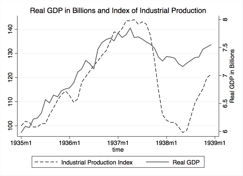
The industrial production variable was obtained from the Federal Reserve. The Federal Reserve’s monthly dataset, indexed to January 1935, measures the real output of all manufacturing, mining, and electric and gas utility facilities located in the United States. The variable is plotted in Figure 9.
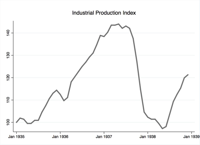
Figure 9. Industrial production indexed to January 1935. Source: See footnote 177.
The search for the alternative regressand, GDP, was more elusive. During the focal time period, GDP had not yet been adopted as a measure of aggregate output. Furthermore, historic measures of output used during the time period are incompatible for use in this study because they are provided only on an annual basis. Luckily, other papers concerned with this time period have addressed the issue of monthly data availability. This study utilizes as the alternative regressand a monthly real GDP variable obtained from the Gordon-Krenn monthly and quarterly dataset for 1913-1954. Figure 10 plots the real GDP variable.
Gordon and Krenn’s dataset provides reliable and important data that is unavailable from traditional sources, like the NBER. Facing the same issue of data availability, Gordon and Krenn converted annual GDP component data to quarterly and monthly intervals, using the Chow-Lin interpolation. For each annual GDP component, Gordon and Krenn used monthly NBER datasets, chosen for their high correlation with the annual GDP component of interest, to ensure an accurate conversion process. Finally, they summed the new monthly component data to provide a measure of monthly GDP.
Although both industrial production and GDP show a clear decline during the Recession, each variable varies significantly in the percent change realized. For comparative purposes, Figure 10 combines industrial production, as shown in Figure 9, and real GDP. During the Recession, the decline in industrial production was greater than that of GDP because the Recession impacted industry most severely. Given the difference in percent change, both indicators are used in order to examine the downturn in a more nuanced manner.
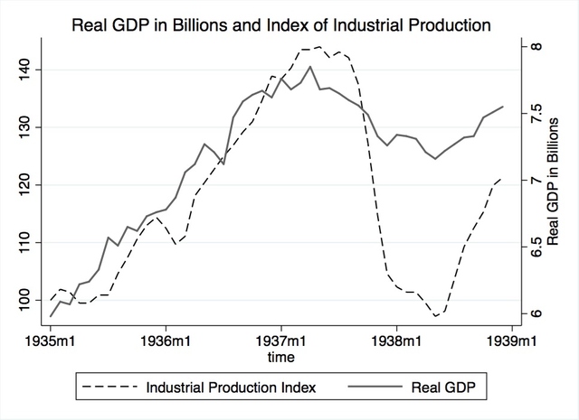
Figure 10. Industrial production index and real GDP in billions, 1935-1938. Source: Refer to footnotes 177 and 178.
The fiscal policy variable used in this study, real government expenditures in 1937 dollars, was obtained from the Gordon and Krenn dataset and is plotted Figure 11. They transformed NBER series 15005, federal budget expenditures, into real terms. Subsequently, they removed the value of transfer payments, like the Soldier’s Bonus, that were included in the original NBER series. They removed transfer payments because their government-spending variable was to be used in calculating monthly GDP. Gordon and Krenn’s dataset is used because it requires no further adjustment. However, there may be need for a dummy variable to account for the large dip in spending that occurred during the first two months of bonus disbursement.
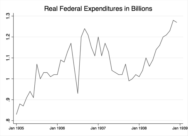
Figure 11. Real federal expenditures in billions. Source: See footnote 178 and 180.
The wage increase caused by the NLRA was historically hypothesized to have contributed to the Recession. Although recent research discounts this view, it is nonetheless important to examine the casual impact, if any, of the NLRA. The search for a wage variable required the fulfillment of two prerequisites:
- The variable must be confined to industries impacted by the NLRA.
- The variable’s NLRA-induced fluctuations shouldn't be overshadowed by wage fluctuations unrelated to the NLRA.
At first glance, the first requirement may seem overly restrictive given the Recession’s national impact. However, it’s important to remember that the manufacturing industry, arguably the most important and largest industry at the time, was directly impacted by NLRA regulations. With this point in mind, the variable search was confined to the manufacturing sector in the interest of excluding wage effects from large but non-regulated industries. Fulfillment of the second requirement is crucial to this study because a wage variable is included to test only the impact of the NLRA-induced wage increases on the economy. A wage variable that fluctuates with non-NLRA factors the interpretation of the NLRA’s impact more difficult.
The variable search started with NBER macrohistory database series 08283, production worker wage cost per unit of output. However, this variable’s denominator, manufacturing output, declined during the Recession to a greater degree than its numerator: wages. The variable is incompatible for use because the NLRA-induced wage increase is not the only factor causing major fluctuations in value.
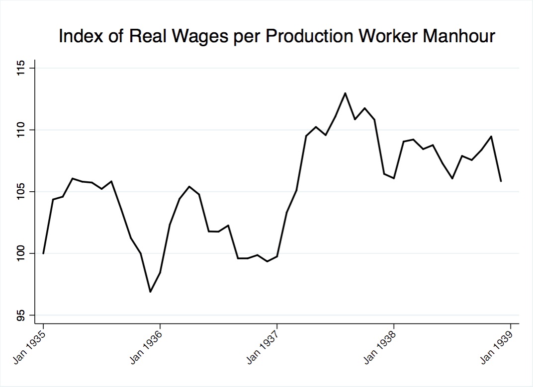
The variable ultimately chosen for use in modeling was wages per hour worked in manufacturing, a slight variation of the aforementioned series, wages per unit output in manufacturing. The new variable was created by dividing the index of real factory payrolls (NBER macrohistory series 08242) by the index of production worker manhours in manufacturing (NBER macrohistory series 08265). Wages per manhours worked, henceforth referred to as the wage variable, was chosen because the variable minimizes fluctuations caused by the Recession, while it maximizes fluctuations caused by the NLRA. The wage variable highlights the impact of the NLRA because it is less reflective of broader changes in the economy. By construction, it provides a clearer understanding of labor costs because wages are considered per unit output realized.
Figure 12 and Figure 13 visualize the desirability of the chosen wage variable. As shown in Figure 12, industrial production, real wages, and manhours worked exhibit a near 1:1 relationship. On the other hand, Figure 13, a plot of wages per manhour worked, shows more nuanced fluctuations. It’s important to note that during the NLRA-impact period, from 1936 to late-1937, the wage variable realizes a 10% increase. The size of the increase is comparable to the increase in manufacturing sector wages reported by Cole and Ohanian and plotted in the previous chapter, Figure 7. The post-1937 plot of the wage variable is also comparable to the post-1937 plateau of manufacturing sector wages in Figure 7.
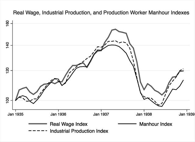
Figure 12. Index of real wages, industrial production, and production worker manhours. Data adapted from: NBER macrohistory database series 08242 and 08265.
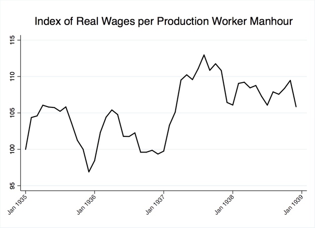
Figure 13. Wage variable used in study, index of real wages per production worker manhours.
Data adapted from: NBER macrohistory database series 08242 and 08265.
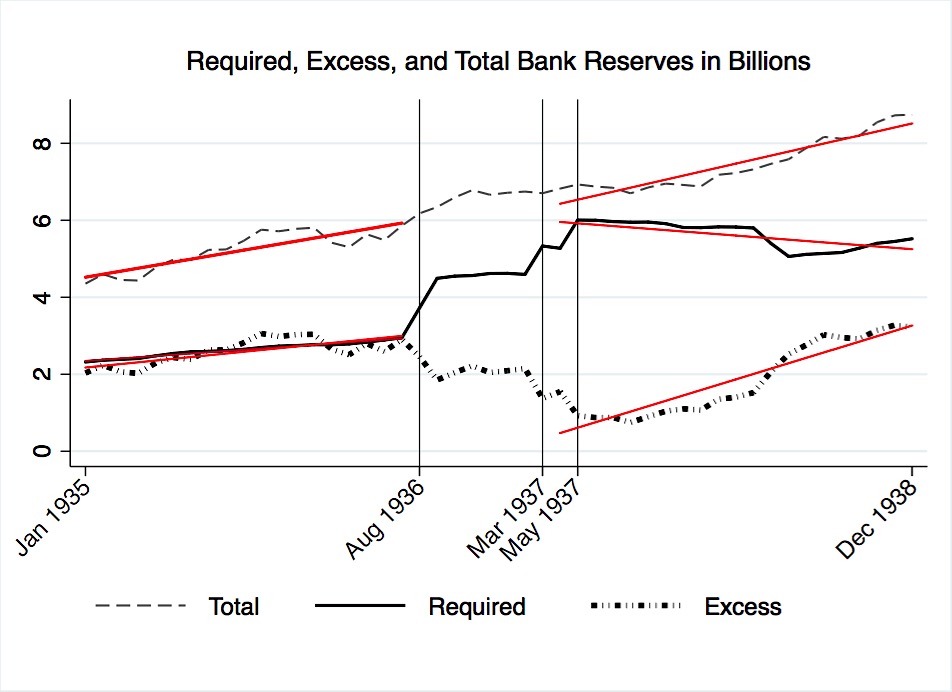
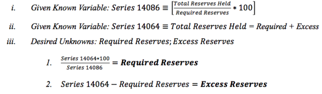
It is necessary to examine the banking sectors’ response to the increased reserve requirements prior to choosing a variable that reflects the impact of monetary policy on the money supply. However, the NBER macrohistory database does not provide distinct datasets for excess and required reserves held. As a workaround, two NBER datasets were used to calculate distinct measures for excess and required reserves. To split the NBER’s total reserves dataset into its excess and required component parts, the equations below were solved for each monthly observation point:
Total reserves, required reserves, and excess reserves are plotted in Figure 14. Vertical lines mark the Federal Reserve’s three reserve requirement increases. For each line plot, a line of best fit is superimposed for the months preceding the Federal Reserve’s first increase in August 1936. Similarly, a line of best fit is added to each plot onwards from April 1937; April is situated one month after the second reserve requirement increase and one month before the third.
Figure 14 shows that banks responded to the reserve requirement increases by further padding their reserves. After the first increase, excess reserves declined as banks shifted funds to required holdings. However, after the third increase, banks started to accumulate excess reserves. Given that total required reserves remained relatively stable after the third increase, and given that total excess reserves increased during the same time, it can be assumed that banks accumulated excess reserves by liquidating assets that would have otherwise been put to alternative use. Clearly, the risk-averse banking sector desired a cushion of excess reserves.
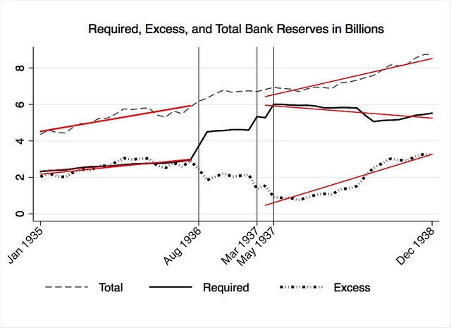
Figure 14. Bank reserves and their trajectories before and after the Fed-mandated increases.
In his paper on the 1937 recession, Velde also concluded that excess reserve accumulation was reactionary. Instead of examining aggregated national data like that used in Figure 14, Velde studied the behavior of banks by member class. He found that central reserve city banks, like those in New York and Chicago, in 1937 were “considerably closer to their [reserve] limit than banks in reserve cities and country banks.” Central reserve city banks faced significantly greater excess reserve depletion than other member banks. This class of member banks was at the forefront of excess reserve accumulation. Therefore, the post-April 1937 positive slope of Figure 14’s excess reserves plot was most greatly influenced by central reserve city bank accumulation.
Although the Federal Reserve succeeded in making excess reserves unusable, banks responded by hoarding as excess even more assets. During the focal time period, the banking sector treated excess reserves not as a pool of money to be utilized, but as a lifeline locked away for use in times of crises. Having confirmed the banking sector’s excess reserve accumulation as reactionary accumulation, the measure of money supply to be used in this study will exclude both required and excess reserves from its sum.
It is the unfortunate reality that some contemporary studies of the Recession utilize standardized measures of the money supply, like M1 or M2, to characterize their variables without explicitly defining the component parts of the measure used. Because contemporary measures of money supply did not exist in the 1930s, it is sometimes difficult to neatly classify long-defunct institutions, like the postal savings bank, under measures crafted for a modern banking system. Adding to the confusion when examining historic studies, the standardized measures in use today were the product of a 1980s redefinition of the existing “M”s. To avoid any confusion, the money supply variable used in this study will not be classified as any current standard measure.
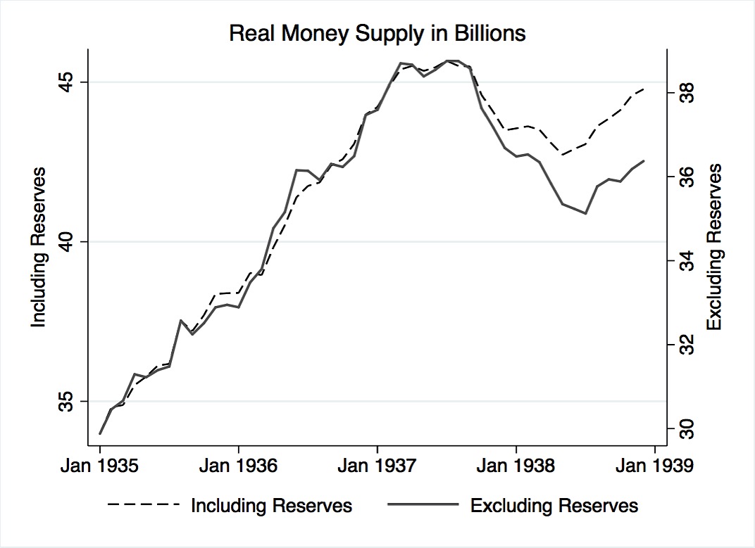
NBER macrohistory database series 14144a, money stock in billions of dollars, is used in the creation of the money supply variable. Series 14144a is the seasonally adjusted sum of currency held by the public, all commercial bank demand deposits, and all commercial bank time deposits. Prior to creating a money supply variable, total reserves held (series 14064) and money stock (series 14144a) were deflated using Gordon and Krenn’s GDP deflator.
Figure 15 plots two possible renditions of money supply. The dashed line plots real money supply, the deflated series 14144a. By construction, the series includes in its sum total reserves held. The solid line plots real money supply excluding real total reserves. As is clear in the post-1937 plot period, the increase in total reserves, caused mainly by an accumulation of new excess reserves, had a negative impact on the already decreasing money supply. Whereas prior to 1937, both line plots in the figure have a near 1:1 relationship, in the months after 1937, money supply exclusive of total reserves decreased to a greater extent than money supply inclusive of reserves. Therefore, the variable used in subsequent modeling is money supply excluding reserves, henceforth referred to only as money supply.
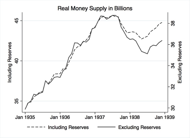
Figure 15. Real money supply including and excluding total reserves. Data adapted from: NBER macrohistory database series 14064 and 14144a.
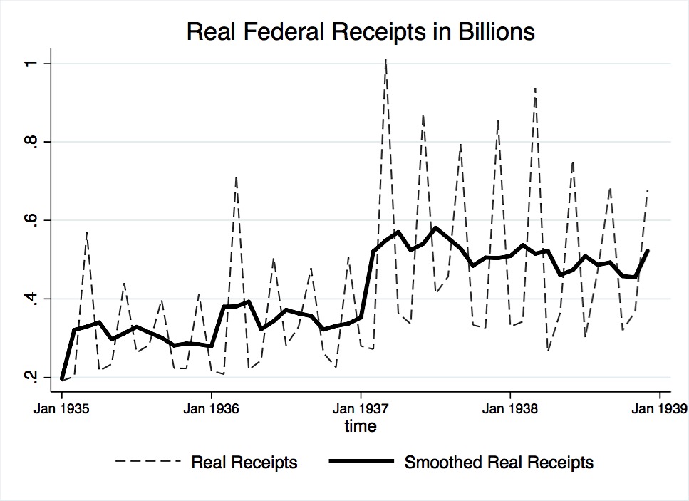
Although not of much interest, a tax variable is used in modeling. NBER series 15004, total federal budget receipts in millions, was chosen for use. The NBER’s dataset was transformed into billions of dollars and deflated using the Gordon and Krenn deflator. Because it was not seasonally adjusted by the NBER, the variable was smoothed using a moving average of the previous, present, and future month. Figure 16 plots real federal budget receipts before and after smoothing.
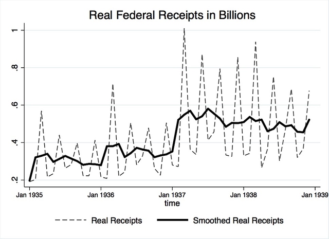
Figure 16. Real federal budget receipts, smoothed and non-adjusted. Source: NBER Series 15004
The variables are log-transformed in order to normalize the data. A log-log model allows for a simple interpretation of the coefficients: a 1% increase in an independent variable leads to a percent change of the regressand that is equivalent to the value of the coefficient output. To gain a better understanding of the variables under consideration, and to aid in model specification, focus was paid to identifying the time-series properties of each variable.
To test for serial correlation of the logged real GDP variable, a correlogram was performed. The correlogram provides two important measures, the autocorrelation and partial autocorrelation functions. The autocorrelation function measures the variable’s correlation with itself at each lag. The partial autocorrelation function, at each lag, is a regression of the variable and that lag, holding all others lags constant. Figure A-1 plots GDP’s autocorrelation function. The plot shows that GDP is significantly correlated with up to three previous years. The plot shows a prolonged and somewhat smooth decay of the autocorrelation function, hinting that the data may be non-stationary. Given the decay of the autocorrelation function, GDP is an autoregressive process.
The partial autocorrelation function of GDP is plotted in Figure A-2. The plot provides a more precise visualization of the autoregressive process. As shown in the figure, when the effect of the first lag is controlled for, the correlation of all other lags is, generally, insignificant. Although the function shows significant correlations at lags 1, 6, 13, 16, and 21, it should be underscored that the function cuts off and remains insignificant for five lags after the first. Given the non-zero partial autocorrelation of the first lag, coupled with the long lag delay before other significant spikes arise, it is assumed that GDP is an AR(1) process. The assumption of an AR(1) process is underscored by Figure A-3, a scatterplot of GDP and its first lag, and Figure A-4, a scatterplot of GDP and its second lag. Both plots have clear upward trends that are usually associated with an autoregressive processes.
Given the very high correlation between the income variable and its lags, coupled with the previous tests that indicate an autoregressive process, the analysis continues by examining the type of autoregressive process seen in GDP. To test for a unit root, a Dickey-Fuller test was performed. The null hypothesis is that the variable contains a unit root. The test was performed and produced an output of -2.841, with the p-value being 0.0526. The low p-value barely misses the 95% significance level, indicating that the null hypothesis cannot be rejected. The test was also performed using an increasing number of lags (5-11). The additional tests confirmed that the null hypothesis couldn’t be rejected. Having confirmed the existence of a unit root, the variable is now said to be a random walk. Further Dickey-Fuller tests were used to specify the type of random walk.
The variable can either be a random walk with drift or without drift. A random walk without drift is a process where the current value of a variable is composed of its past values plus an error term. A random walk with drift is, essentially, a random walk with an added constant parameter. GDP was tested for drift and test’s p-value was 0.0034. The null hypothesis can be rejected, and the results held with the use of varying lag lengths. GDP is a random walk without drift. GDP, a variable confirmed to be a random walk without drift, was also tested for a deterministic time trend. The test statistic output was -1.642 with a p-value of .7754. GDP is a unit root around a deterministic time trend. A regression of GDP and time further confirmed the existence of a time trend. Because the GDP variable is non-stationary, it is used in modeling in its differenced form.
The tests performed above were repeated on the industrial production variable. Figure A-5, the autocorrelation function of industrial production, shows a steep but smooth decay. Figure A-6, the partial autocorrelation function, is significant at lags 1, 2, with some peaks after lag 10. These graphs suggest that industrial production is an autoregressive. Next, a Dickey Fuller test for unit root was performed. With and without varying lags included, the test output indicated a unit root. The test was repeated with trend added. At varying lags, the test output confirmed the existence of a unit root with a deterministic time trend. However, the test for drift produced inconclusive results. Therefore, the assumption is made that industrial production is a unit root with a deterministic time trend. Like the GDP variable, industrial production will be differenced when used as a regressand. Given that both possible dependent variables are used in differenced form, independent variables will also be differenced to make the interpretation of model results simpler.
To consider whether industrial production or GDP should be used as the dependent variable, each regressor was individually regressed by up to 4 differenced lags on the two possible regressands. After each regression, a Durbin-Watson test and Breusch-Godfrey test was performed to look for autocorrelation between the regressor variable and the regressand under consideration. The simple regression results are reported in Table A-4 and the Breusch-Godfrey test outputs are reported in Table A-5. Overwhelmingly, when each independent variable was individually regressed on industrial production, the Durbin-Watson test and the Breusch-Godfrey test indicated autocorrelation of the error terms. Therefore, GDP was chosen as the dependent variable to be used in modeling.
The first model used included 3 differenced lags of each independent variable. The results of Model 1 are reported in Table A-1, alongside results for models soon to be discussed. Due to the use of lagged variables in Model 1, the Breusch-Godfrey (BG) test was the prime test of interest. Unlike the Durbin-Watson test, the BG test allows for lagged dependent variables and tests for higher order autoregressive processes. The test output is reported in Table A-2. Based on the reported p-values, the null hypothesis that serial correlation does not exist, was not rejected. In other words, the assumption was made that serial correlation does not exist.
Before further analyzing results, Model 1 residuals were tested for problems. Figure A-7 plots residuals against fitted values. The graph shows a random scatter, a preliminary indicator that the results were favorable. Furthermore, Figure A-8 shows that the residuals are somewhat normally distributed. It should be noted that Figure A-9, a scatterplot of the residuals against time, appears to be random with no patterns. The autocorrelation function, Figure A-10, shows no lags of significance, and the partial autocorrelation function, Figure A-11, shows no lags of significance. A runs test indicated that the residuals had 24 runs. The p-value output provided was 0.72; the null hypothesis is that the residuals were produced from a random process, which was not rejected. This test further indicated that autocorrelation was not a problem in the model. Finally, Dickey Fuller tests without drift, with drift, and with trend were performed on the residuals. All three tests had p-value outputs of 0.00, thereby raising no concerns regarding a unit root of the residuals. Based on testing of the residuals, the standard error outputs provided in Model 1 were not biased.
To continue improving the model, the wage variable was incorporated in Model 1.1 in its unlogged form. The output of Model 1.1 is reported in Table A-1. The fit of the model improved slightly and the regression results remained comparable to Model 1. Given this slight improvement, coupled with the favorable BG test results reported in Table A-2, the wage variable was retained for use in its unlogged form.
Due to their removal of the Soldier’s Bonus impact, the Gordon and Krenn data for government spending declines sharply in June 1936 and July 1936. In Model 2, a time dummy variable for these two months was included to remove a potential source of bias. The inclusion of the dummy variable removed a slight bias from regression results; however, the dummy variable was insignificant in all models.
Model 3 builds upon Model 2 by using a different measure of the money supply variable. In line with other studies of the Recession, the money supply variable in Model 3 was changed to include total reserves. The results of this regression, with all other variables kept unchanged from Model 2, are reported in Table A-3. Although the fiscal policy coefficient does not change as a result of the variable change, the coefficient of money supply increased from .42 in Model 2 to .61 in Model 3. These results should be considered surprising because the variable, having strayed from the argument that reserve hoarding decreased money supply, has now a greater impact in the regression. The money supply coefficients in Model 3 are counterintuitive and the results suggest that other studies, utilizing measures inclusive of reserves, may have inadvertently inflated the role of money supply. Given that the government-spending coefficient remained unchanged in Model 3 and given the reasons for excluding reserves, the next model retained money supply exclusive of reserves.
The final model examined, Model 4, was a cleaned regression of only the significant variable-level lags. Reported in Table A-3, the fit of this regression remained high while the variable coefficients and beta coefficients continued to mirror those previously modeled. Furthermore, this model’s BG test, as reported in Table A-2, produced an output even more favorable than that of the other models. Model 4’s residual plots, Figure A- 12 to Figure A- 15, were all favorable.Continued on Next Page »
An Act to Diminish the Causes of Labor Disputes Burdening or Obstructing Interstate and Foreign Commerce, to Create a National Labor Relations Board, and for Other Purposes., Pub. L. No. 74-198, Stat. (July 5, 1935). Accessed January 16, 2015. http://research.archives.gov/description/299843.
An act to provide adjusted compensation for veterans of the World War, and for other purposes., H.R. 10874, 67th Cong., 2d Sess. (1922).
Adjusted Compensation Payment Act, ch. 32, 49 Stat. 1099-1102 (Jan. 27, 1936).
Allen, William R. "Irving Fisher, F. D. R., and the Great Depression." History of Political Economy 9, no. 4 (1977): 560-87. http://EconPapers.repec.org/RePEc:hop:hopeec:v:9:y:1977:i:4:p:560-587.
Baker, Nancy. "Abel Meeropol (a.k.a. Lewis Allan): Political Commentator and Social Conscience." American Music 20, no. 1 (Spring 2002): 25-79.
Barber, William J. From New Era to New Deal: Herbert Hoover, the Economists, and American Economic Policy, 1921-1933. Cambridge: Cambridge University Press, 1988.
Black, Conrad. Franklin Delano Roosevelt: Champion of Freedom. New York: Public Affairs, 2003.
Board of Governors of the Federal Reserve System (US), Industrial Production Index[INDPRO], retrieved from FRED, Federal Reserve Bank of St. Louis https://research.stlouisfed.org/fred2/series/INDPRO/, April 4, 2015.
Brown, E. Cary. "Fiscal Policy in the 'Thirties: A Reappraisal." The American Economic Review 46, no. 5 (December 1956): 857-79.
The Brownsville Herald (Brownsville, TX). "Prices." April 2, 1937, 1.
The Brownsville Herald (Brownsville, TX). "Public Funds Will Control High Prices?" April 4, 1937, 1-2.
Burns, Arthur F., and Wesley C. Mitchell. Measuring Business Cycles. Studies in Business Cycles 2. New York: National Bureau of Economic Research, 1946.
Cargill, Thomas F., and Thomas Mayer. "The Effect of Changes in Reserve Requirements during the 1930s: The Evidence from Nonmember Banks." The Journal of Economic History 66, no. 2 (June 2006): 417-32.
Cole, Harold L., and Lee E. Ohanian. "New Deal Policies and the Persistence of the Great Depression: A General Equilibrium Analysis." Journal of Political Economy 112, no. 4 (August 2004): 779-816. Accessed January 16, 2015. doi:10.1086/421169.
Complete Set of Speech Drafts. Volume 97: November 10, 1937. Diaries of Henry Morgenthau, Jr. Franklin D. Roosevelt Presidential Library & Museum, Hyde Park, NY.
Conference to Talk Over Plans, 9/13/37. Volume 95: November 10, 1937; Page 1. Diaries of Henry Morgenthau, Jr. Franklin D. Roosevelt Presidential Library & Museum, Hyde Park, NY.
"Document 50: February 28, 1938, Letter with Attachments, To: Keynes From: Roosevelt." In FDR's Response to Recession, edited by George McJimsey, 303-12. Vol. 26 of Documentary History of the Franklin D. Roosevelt Presidency. N.p.: University Publications of America, 2005.
Draft Letter to FDR. November 3, 1937. Volume 94: November 1-November 10, 1937; Page 47. The Diaries of Henry Morgenthau, Jr. Franklin D. Roosevelt Presidential Library & Museum, Hyde Park, NY.
Dutcher, Rodney. "Behind the Scenes in Washington." The Brownsville Herald (Brownsville, TX), April 2, 1937, 4.
Edsforth, Ronald. The New Deal: America's Response to the Great Depression. Malden, MA: Blackwell Publishers, 2000.
Eggertsson, Gauti B. Great Expectations and the End of the Depression. Staff Report no. 234. N.p.: Federal Reserve Bank of New York, 2005.
———. "Great Expectations and the End of the Depression." American Economic Review 98, no. 4 (September 2008): 1476-516. doi:10.1257/aer.98.4.1476.
Eggertsson, Gauti B., and Benjamin Pugsley. "The Mistake of 1937: A General Equilibrium Analysis." Monetary and Economic Studies 24, nos. S-1 (December 2006): 151-90.
Eichengreen, Barry. "The U.S. Capital Market and Foreign Lending, 1920–1955." In Developing Country Debt and Economic Performance: The International Financial System, by Susan Margaret Collins and Jeffrey Sachs, 107-56. Vol. 1. Chicago: University of Chicago Press, 1989. Previously published as "Til Debt Do Us Part: The U.S. Capital Market and Foreign Lending, 1920-1955." NBER Working Paper W2394. http://www.nber.org/chapters/c8988.
"FDR: From Budget Balancer to Keynesian, A President's Evolving Approach to Fiscal Policy in Times of Crisis." Franklin D. Roosevelt Presidential Library and Museum. http://www.fdrlibrary.marist.edu/aboutfdr/budget.html.
Federal Reserve Board. Tenth Annual Report of the Federal Reserve Board: Covering Operations for the Year 1923. Washington: Government Printing Office, 1924. Accessed November 23, 2014. https://fraser.stlouisfed.org/docs/publications/arfr/1920s/arfr_1923.pdf.
Fisher, Irving. Booms and Depressions: Some First Principles. New York: Adelphi, 1932.
———. "The Debt-Deflation Theory of Great Depressions." Econometrica 1, no. 4 (October 1933): 337-57. DOI:10.2307/1907327.
———. "Dollar Stabilization." In Encyclopedia Britannica, 852-53. Vol. XXX. http://www.econlib.org/library/Essays/fshEnc1.html.
———. "Mathematical Investigations in the Theory of Value and Prices." Transactions of the Connecticut Academy of Arts and Sciences 9 (1892): 1-124.
———. "Our Unstable Dollar and the So-Called Business Cycle." Journal of the American Statistical Association 20, no. 150 (June 1925): 179-202. doi:10.2307/2277113.
———. "Stabilizing Price Levels." The New York Times, September 2, 1923, sec. XX, 10.
———. "Why Has the Doctrine of Laissez Faire Been Abandoned?" Science, n.s., 25, no. 627 (January 4, 1907): 18-27. http://www.jstor.org/stable/1633692.
Friedman, Milton, Paul A. Samuelson, and Henry Wallich. "How the Slump Looks to Three Experts." Newsweek, May 25, 1970, 78-79. Accessed November 23, 2014. http://hoohila.stanford.edu/friedman/newsweek.php.
Friedman, Milton, and Anna Jacobson Schwartz. A Monetary History of the United States 1867-1960. 9th ed. Princeton: Princeton University Press, 1993.
Gordon, Robert J., and Robert Krenn. "New Gordon-Krenn quarterly and monthly data set for 1913-54." Unpublished raw data, Northwestern University, n.d. Accessed March 30, 2015. http://faculty-web.at.northwestern.edu/economics/Gordon/researchhome.html.
Hearings Before the Banking, Housing, and Urban Affairs (2009) (statement of Lee E. Ohanian). Accessed January 25, 2015. http://www.banking.senate.gov/public/index.cfm?FuseAction=Files.View&FileStore_id=6cce4fbb-e7cd-4699-8892-9c5d1285e871.
Hemingway, Ernest. "Who Murdered the Vets?" The New Masses, September 17, 1935, 9-10. Accessed March 10, 2015. http://www.unz.org/Pub/NewMasses-1935sep17-00009.
Hobsbawm, E. J. Industry and Empire: The Birth of the Industrial Revolution. Edited by Chris Wrigley. New York: New Press, 1999. Originally published as Industry and Empire: An Economic History of Britain Since 1750 (London: Weidenfeld & Nicolson, 1968).
Jones & Laughlin Steel Corp. v. NLRB, 301 U.S. (1937). Accessed January 16, 2015. https://supreme.justia.com/cases/federal/us/301/1/case.html.
Kahn, Richard. "The Relation of Home Investment to Unemployment." The Economic Journal 41, no. 162 (June 1931): 173-98.
Keynes, John Maynard. "Chapter 24: Concluding Notes on the Social Philosophy towards Which the General Theory Might Lead." In The General Theory of Employment, Interest, and Money.
———. "The Great Slump of 1930." The Nation and Athenaeum 48 (December 20, 1930): 402.
———. "The Great Slump of 1930 II." The Nation and Athenaeum 48 (December 27, 1930): 427-28.
———. A Tract on Monetary Reform. 1923. Reprint, London: Macmillan, 1924.
Kindleberger, Charles Poor. The World in Depression, 1929-1939. Berkeley: University of California Press, 1973.
May, Dean L. From New Deal to New Economics: The Liberal Response to the Recession. Edited by Frank Freidel. Modern American History. New York: Garland Publishing, 1981.
Mehrotra, Ajay K. "Edwin R.A. Seligman and the Beginnings of the U.S. Income Tax." Tax Notes, November 14, 2005, 933-50.
Nasar, Sylvia. Grand Pursuit: The Story of Economic Genius. New York: Simon & Schuster, 2011.
NBER. The End of the Great Depression 1939-41: Policy Contributions and Fiscal Multipliers. By Robert J. Gordon and Robert Krenn. Working Paper no. 16380. 2010. Accessed March 30, 2015. doi:10.3386/w16380.
The New York Times. "Bonus Bill Becomes Law." January 28, 1936, Late City edition, 1. Accessed March 8, 2015. http://timesmachine.nytimes.com/timesmachine/1936/01/28/87903226.html?pageNumber=1.
The New York Times. "Both Coasts Threatened." September 3, 1935, Late City edition, 1. Accessed March 8, 2015. http://timesmachine.nytimes.com/timesmachine/1935/09/03/issue.html.
The New York Times. "Fisher Sees Stocks Permanently High." October 16, 1929, 8.
The New York Times. "Link Bonus Issue to Florida Deaths." September 15, 1935, Late City edition, N6. Accessed March 8, 2015. http://timesmachine.nytimes.com/timesmachine/1935/09/15/93707816.html?pageNumber=99.
The New York Times. "The Stock Market." October 20, 1937, Late City edition, 22. Accessed March 8, 2015. http://timesmachine.nytimes.com/timesmachine/1937/10/20/103216107.html?pageNumber=22.
The New York Times. "Veteran's Camp Wrecked by Storm." September 4, 1935, Late City edition, 1. Accessed March 8, 2015. http://timesmachine.nytimes.com/timesmachine/1935/09/04/93481928.html.
The New York Times. "Veterans Lead Fatalities. Only 11 of 192 Reported as Left Alive in One Florida Camp." September 5, 1935, Late City edition, 1. Accessed March 8, 2015. http://timesmachine.nytimes.com/timesmachine/1935/09/05/93482496.html?pageNumber=1.
Office of the Secretary of the Senate, Presidential Vetoes, 1789-1988, S. Doc. No. 102-12 (1992). Accessed March 8, 2015. http://www.senate.gov/reference/resources/pdf/presvetoes17891988.pdf.
"131 'I Pledge You—I Pledge Myself to a New Deal for the American People.' the Governor Accepts the Nomination for the Presidency, Chicago, Ill. July 2, 1932." In The Genesis of the New Deal, 1928-1932, 647-58. Vol. 1 of The Public Papers and Addresses of Franklin D. Roosevelt. New York: Random House, 1938.
Papadimitriou, Dimitri B., and Greg Hannsgen. Lessons from the New Deal: Did the New Deal Prolong or Worsen the Great Depression? Working Paper no. 581. Annandale-on-Hudson, NY: Levy Economics Institute of Bard College, 2009.
Personal Memo. October 19, 1937. Volume 92: October 12-October 19, 1937; Page 229. The Diaries of Henry Morgenthau, Jr. Franklin D. Roosevelt Presidential Library & Museum, Hyde Park, NY.
"Press Conference #425-15." January 14, 1938. Press Conferences of President Franklin D. Roosevelt, 1933-1945. Franklin D. Roosevelt Presidential Library & Museum, Hyde Park, NY.
"Press Conference #434." February 15, 1938. Press Conferences of President Franklin D. Roosevelt, 1933-1945. Franklin D. Roosevelt Presidential Library & Museum.
Press Conference #401-1. October 8, 1937. Press Conferences of President Franklin D. Roosevelt, 1933-1945. Franklin D. Roosevelt Presidential Library & Museum, Hyde Park, NY.
"Press Conference #405-5." October 22, 1937. Press Conferences of President Franklin D. Roosevelt, 1933-1945. Franklin D. Roosevelt Presidential Library & Museum, Hyde Park, NY.
"Press Conference #409-7." November 9, 1937. Press Conferences of President Franklin D. Roosevelt, 1933-1945. Franklin D. Roosevelt Presidential Library & Museum, Hyde Park, NY.
"Press Conference #415-8." December 10, 1937. Press Conferences of President Franklin D. Roosevelt, 1933-1945. Franklin D. Roosevelt Presidential Library & Museum, Hyde Park, NY.
"Press Conference #416-4." December 14, 1937. Press Conferences of President Franklin D. Roosevelt, 1933-1945. Franklin D. Roosevelt Presidential Library & Museum, Hyde Park, NY.
"Press Conference #357." April 2, 1937. Page 239. Press Conferences of President Franklin D. Roosevelt, 1933-1945. Franklin D. Roosevelt Presidential Library & Museum.
Romer, Christina D. "Lessons from the Great Depression for Economic Recovery in 2009." Speech presented at Brookings Institution, Washington D.C., March 9, 2009. Accessed April 21, 2015. http://www.brookings.edu/~/media/events/2009/3/09-lessons/0309_lessons_romer.pdf.
———. "Spurious Volatility in Historical Unemployment Data." Journal of Political Economy 94, no. 1 (February 1986): 1-37. http://www.jstor.org/stable/1831958.
———. "What Ended the Great Depression?" The Journal of Economic History 52, no. 4 (December 1992): 757-84.
Roose, Kenneth D. The Economics of Recession and Revival: An Interpretation of 1937-38. Yale Studies in Economics 2. New Haven: Yale University Press, 1954.
———. "The Recession of 1937-38." Journal of Political Economy 56, no. 3 (June 1948): 239-48. Accessed January 26, 2015. http://www.jstor.org/stable/1825772.
———. "The Role of Net Government Contribution to Income in the Recession and Revival of 1937-38." The Journal of Finance 6, no. 1 (March 1951): 1-18. DOI:10.1111/j.1540-6261.1951.tb04437.x.
Roosevelt, Franklin D. "Annual Budget Message to Congress." Address, January 7, 1937. The American Presidency Project. http://www.presidency.ucsb.edu/ws/?pid=15337.
———. "Annual Message to Congress." Address, January 6, 1937. The American Presidency Project. http://www.presidency.ucsb.edu/ws/?pid=15336.
———. "Fireside Chat on Banking." Speech, March 12, 1933. The American Presidency Project. http://www.presidency.ucsb.edu/ws/?pid=14540.
———. "Message to Congress Recommending Legislation, November 5, 1937." The American Presidency Project. http://www.presidency.ucsb.edu/ws/?pid=15496.
———. "Proclamation 2040 - Bank Holiday." The American Presidency Project. http://www.presidency.ucsb.edu/ws/?pid=14485.
———. "Proclamation 2039 - Declaring Bank Holiday." The American Presidency Project. http://www.presidency.ucsb.edu/ws/?pid=14661.
———. "60 - Message to Congress on Appropriations for Work Relief for 1938. April 20, 1937." The American Presidency Project. Accessed March 19, 2015. http://www.presidency.ucsb.edu/ws/?pid=15393.
———. "Statement Summarizing the 1938 Budget, October 19, 1937." The American Presidency Project. Accessed March 22, 2015. http://www.presidency.ucsb.edu/ws/?pid=15486.
Schumpeter, Joseph A. "Chapter 5.4: Unemployment and the ‘State of the Poor’." In History of Economic Analysis, 258-63. Edited by Elizabeth B. Schumpeter. New York: Oxford University Press, 1954.
Shlaes, Amity. The Forgotten Man: A New History of the Great Depression. New York: Harper Collins, 2007.
Smith, Adam. An Inquiry into the Nature and Causes of the Wealth of Nations. Edited by Edwin Cannan. 5th ed. 1776. Reprint, London: Methuen & Co., 1904. http://www.econlib.org/library/Smith/smWN.html.
Telser, Lester G. "Higher Member Bank Reserve Ratios in 1936 and 1937 Did Not Cause the Relapse into Depression." Journal of Post Keynesian Economics 24, no. 2 (Winter 2001-2): 205-16.
———. "The Veterans' Bonus of 1936." Journal of Post Keynesian Economics 26, no. 2 (Winter 2003-4): 227-43.
Three Parts of Speech as Decided Upon, 10/28/37. Volume 95: November 10, 1937; Page 261. Diaries of Henry Morgenthau, Jr. Franklin D. Roosevelt Presidential Library & Museum, Hyde Park, NY.
The Times-Picayune (New Orleans, LA). "A Cloud That's Dragonish." January 8, 1937, 12.
The Times-Picayune (New Orleans, LA). "Industry Pushes up after Holiday Lull; Steel Leads." January 11, 1937, 18.
Transcript of Call between Morgenthau and Burgess. October 19, 1937. Volume 92: October 12-October 19, 1937; Page 222. The Diaries of Henry Morgenthau, Jr. Franklin D. Roosevelt Presidential Library & Museum, Hyde Park, NY.
Transcript of Phone Call between Morgenthau and FDR. October 20, 1937. Volume 93: October 20-October 31, 1937; Page 21. The Diaries of Henry Morgenthau, Jr. Franklin D. Roosevelt Presidential Library & Museum, Hyde Park, NY.
United States Senate Special Committee on the Termination of the National Emergency. Emergency Powers Statutes: Provisions of Federal Law Now in Effect Delegating to the Executive Extraordinary Authority in Time of National Emergency. Report no. 93-549. Washington: Government Printing Office, 1973.
U.S. Department of Commerce Bureau of Foreign and Domestic Commerce. Statistical Abstract of the United States 1934. Washington: Government Printing Office, 1934. Accessed November 23, 2014. https://fraser.stlouisfed.org/docs/publications/stat_abstract/1930s/sa_1934.pdf.
Velde, François. "The Recession of 1937—A Cautionary Tale." Economic Perspectives 33, no. 4 (2009): 16-37.
Wood, Howard. "Stocks Crash to New Lows; Selling Swamps Market; Blame Federal Policies." Chicago Daily Tribune, October 19, 1937, Final edition, 1. Accessed March 10, 2015. http://archives.chicagotribune.com/1937/10/19/page/1/article/stocks-crash-to-new-lows.
World War Adjusted Compensation Act, ch. 157, 43 Stat. 121-131 (May 19, 1924). Accessed March 7, 2015. http://www.loc.gov/law/help/statutes-at-large/68th-congress/c68.pdf.
Yale University. "Past Presidents." Office of the President. Accessed December 7, 2014. http://president.yale.edu/past-presidents.
Endnotes
- Real GDP is a measure of economic output that is adjusted for price changes at each observation year. The values in Figure 1 are in terms of 1937 dollars.
- The data was made relative to the pre-Depression peak in industrial production, which occurred in the year 1929. In other words, the data was adjusted so that the 1929 peak equals 100%.
- Barber, From New Era to New Deal, 118.
- Ibid.,195.
- Ibid., 36.
- Kindleberger, The World in Depression, 56.
- Eichengreen, "The U.S. Capital Market," in Developing Country Debt and Economic, 1:122.
- Ibid.
- Ibid., 1:124.
- Barber, From New Era to New Deal, 72.
- Ibid., 73.
- U.S. Department of Commerce Bureau of Foreign and Domestic Commerce, Statistical Abstract of the United, 279.
- According to data obtained from the BEA, GDP in 1929 was $104.6 Billion and 2014 Q2 GDP is $16,010 Billion.
- Federal Reserve Board, Tenth Annual Report of the Federal, 34.
- Friedman and Schwartz, A Monetary History of the United, 254.
- Fisher Sees Stocks Permanently High,” The New York Times, October 16, 1929.
- Friedman, Samuelson, and Wallich, "How the Slump Looks to Three Experts," Newsweek, May 25, 1970.
- The money supply refers to money available for use and circulating in the economy. Varying standardized measures of the money supply exist, from most liquid measurement of money to least liquid.
- Friedman and Schwartz, A Monetary History of the United, 300.
- Ibid., 308.
- Ibid., 310.
- Edsforth, The New Deal: America's, 43.
- Ibid., 40.
- Friedman and Schwartz, A Monetary History of the United, 313.
- Ibid., 315-317.
- Ibid., 322.
- Ibid., Table A-1, 713.
- Black, Franklin Delano Roosevelt: Champion, 269.
- Roosevelt, "Proclamation 2039 - Declaring," The American Presidency Project.
- Roosevelt, "Proclamation 2040 - Bank," The American Presidency Project.
- United States Senate Special Committee on the Termination of the National Emergency, Emergency Powers Statutes: Provisions, 4-5.
- Roosevelt, "Fireside Chat on Banking," The American Presidency Project.
- Friedman and Schwartz, A Monetary History of the United, 311.
- Ibid., 312.
- Hobsbawm, Industry and Empire: The Birth, 190.
- Say’s Law is the defunct notion that production is itself the source of demand. An individual producer is paid for their services and that payment is used to purchase other goods.
- Keynes, "The Great Slump of 1930," 402.
- Nasar, Grand Pursuit: The Story, 323.
- "131 'I Pledge You—I," in The Genesis of the New Deal, 651.
- Ibid., 652.
- Ibid., 658.
- Schumpeter, "Unemployment and the ‘State of the Poor’," inHistory of Economic Analysis.
- A concise history of Progressive-Era economic policy reform efforts, specifically that of public finance, is provided in: Ajay K. Mehrotra, "Edwin R.A. Seligman and the Beginnings of the U.S. Income Tax,"Tax Notes, November 14, 2005.
- Keynes, "The Great Slump of 1930," 402.
- Ibid.
- Keynes, "The Great Slump of 1930, II" 428.
- Smith, An Inquiry into the Nature, IV.2.9.
- Nasar, Grand Pursuit: The Story, 149.
- "Past Presidents," Office of the President.
- Nasar, Grand Pursuit: The Story, 150.
- Ibid., 151.
- Ibid.
- Fisher, "Why Has the Doctrine," 27.
- Nasar, Grand Pursuit: The Story, 283.
- Keynes, A Tract on Monetary, 187.
- Fisher, "Dollar Stabilization.," in Encyclopedia Britannica, XXX.
- Friedman and Schwartz, A Monetary History of the United, 206.
- Ibid., 226-233.
- Romer, "Spurious Volatility in Historical," 31.
- Nasar, Grand Pursuit: The Story, 301.
- Irving Fisher, "Stabilizing Price Levels," The New York Times, September 2, 1923.
- Fisher, "Our Unstable Dollar and the So-Called," 201.
- Fisher, "The Debt-Deflation Theory of Great," 342.
- Fisher, Booms and Depressions: Some, 142.
- Allen, "Irving Fisher, F. D. R., and the Great," 576.
- Ibid., 562.
- Ibid., 580-581.
- Ibid., 577.
- Ibid., 565.
- Ibid., 565.
- Fisher’s latter comment is in regards to the 17% increase in nominal wages between November 1936 and November 1937, as measured by the Bureau of Labor Statistics and the National Industrial Conference Board (Velde, "The Recession of 1937—A," 29).
- Nasar, Grand Pursuit: The Story, 319.
- Ibid., 326.
- Ibid., 324.
- Richard Kahn, "The Relation of Home Investment to Unemployment," The Economic Journal 41, no. 162 (June 1931)
- "FDR: From Budget Balancer to Keynesian,” Franklin D. Roosevelt Presidential Library and Museum, http://www.fdrlibrary.marist.edu/aboutfdr/budget.html.
- Kindleberger, The World in Depression, 262.
- An act to provide adjusted compensation for veterans of the World War, and for other purposes., H.R. 10874, 67th Cong., 2d Sess. (1922). Office of the Secretary of the Senate, Presidential Vetoes, 1789-1988, S. Doc. No. 102-12 (1992), 225.
- Ibid., 228.
- World War Adjusted Compensation Act, ch. 157, 43 Stat. 121-131 (May 19, 1924).
- "Both Coasts Threatened," The New York Times, September 3, 1935.
- "Veteran's Camp Wrecked by Storm," The New York Times, September 4, 1935.
- "Veterans Lead Fatalities,” The New York Times, September 5, 1935.
- "Link Bonus Issue to Florida Deaths," The New York Times, September 15, 1935.
- Nancy Baker, "Abel Meeropol (a.k.a. Lewis Allan): Political Commentator and Social Conscience," American Music 20, no. 1 (Spring 2002): 45.
- Hemingway, "Who Murdered the Vets?," The New Masses, September 17, 1935.
- Adjusted Compensation Payment Act, ch. 32, 49 Stat. 1099-1102 (Jan. 27, 1936).
- "Bonus Bill Becomes Law," The New York Times, January 28, 1936.
- For a detailed analysis of the Soldier’s Bonus expansionary effect, consult: Telser, "The Veterans' Bonus of 1936,"Journal of Post Keynesian Economics26, no. 2 (Winter 2003-4).
- Eggertsson and Pugsley, "The Mistake of 1937," 174.
- Roosevelt, "Annual Message to Congress, January 6, 1937,” The American Presidency Project.
- Roosevelt, "Annual Budget Message to Congress," The American Presidency Project.
- "Press Conference #357," April 2, 1937, Page 239, Press Conferences of President Franklin D. Roosevelt, 1933-1945, Franklin D. Roosevelt Presidential Library & Museum.
- Data source: Board of Governors of the Federal Reserve System (US), Industrial Production Index[INDPRO], retrieved from FRED, Federal Reserve Bank of St. Louis.
- "The Stock Market," The New York Times, October 20, 1937.
- Howard Wood, "Stocks Crash to New Lows,” Chicago Daily Tribune, October 19, 1937.
- "The Stock Market," The New York Times, October 20, 1937.
- Personal Memo, October 19, 1937, Volume 92: October 12-October 19, 1937; Page 229, The Diaries of Henry Morgenthau, Jr., Franklin D. Roosevelt Presidential Library & Museum, Hyde Park, NY.
- Transcript of Call between Morgenthau and FDR. October 19, 1937, Volume 92: October 12-October 19, 1937; Page 230, The Diaries of Henry Morgenthau, Jr., Franklin D. Roosevelt Presidential Library & Museum, Hyde Park, NY.
- Transcript of Call between Morgenthau and Burgess, October 19, 1937, Volume 92: October 12-October 19, 1937; Page 222, The Diaries of Henry Morgenthau, Jr., Franklin D. Roosevelt Presidential Library & Museum, Hyde Park, NY.
- Transcript of Phone Call between Morgenthau and FDR, October 20, 1937, Volume 93: October 20-October 31, 1937; Page 21, The Diaries of Henry Morgenthau, Jr., Franklin D. Roosevelt Presidential Library & Museum, Hyde Park, NY.
- Draft Letter to FDR, November 3, 1937, Volume 94: November 1-November 10, 1937; Page 47, The Diaries of Henry Morgenthau, Jr., Franklin D. Roosevelt Presidential Library & Museum, Hyde Park, NY.
- Roosevelt, "60 - Message to Congress," The American Presidency Project.
- Press Conference #401-1.
- Press Conference #405-5.
- Roosevelt, "Statement Summarizing the 1938," The American Presidency Project.
- Press Conferences #409-7; #415-8; #416-4.
- Press Conference #425-15.
- "A Cloud That's Dragonish,"The Times-Picayune(New Orleans, LA), January 8, 1937, 12.
- "Industry Pushes up after Holiday Lull; Steel Leads,"The Times-Picayune(New Orleans, LA), January 11, 1937, 18.
- Rodney Dutcher, "Behind the Scenes in Washington,"The Brownsville Herald(Brownsville, TX), April 2, 1937,4.
- This small, local, newspaper featured during the same week at least two in-depth articles focused on analysis of policy, not only news: "Public Funds Will Control High Prices?,"The Brownsville Herald(Brownsville, TX), April 4, 1937,1-2. "Prices,"The Brownsville Herald(Brownsville, TX), April 2, 1937,1.
- Conference to Talk Over Plans, 9/13/37, Volume 95: November 10, 1937; Page 1, Diaries of Henry Morgenthau, Jr., Franklin D. Roosevelt Presidential Library & Museum, Hyde Park, NY.
- Three Parts of Speech as Decided Upon, 10/28/37, Volume 95: November 10, 1937; Page 261, Diaries of Henry Morgenthau, Jr., Franklin D. Roosevelt Presidential Library & Museum, Hyde Park, NY.
- Shlaes,The Forgotten Man: A New History, 341-342.
- Complete Set of Speech Drafts, Volume 97: November 10, 1937; Page 149, Diaries of Henry Morgenthau, Jr., Franklin D. Roosevelt Presidential Library & Museum, Hyde Park, NY.
- Ibid., 142.
- Ibid., 143.
- Roosevelt, "Message to Congress Recommending," The American Presidency Project.
- "Document 50: February 28, 1938, Letter with attachments, To: Keynes From: Roosevelt," in FDR's Response to Recession, ed. George McJimsey, vol. 26, Documentary History of the Franklin D. Roosevelt Presidency (University Publications of America, 2005), 307.
- Ibid., 312.
- Roose, "The Recession of 1937-38," 239.
- Roose, "The Role of Net Government," 1.
- Personal Income is income received by individuals, non-profit institutions, private trust funds, and private pension funds. It is the sum of wages, labor income, rental income, interest, dividends, and transfer payments. Source: National Income and Product Statistics of the United States 1929-46, US Dept. of Commerce, 1946, p. 53-54. Net Gvt. Contribution to Income is a breakdown of measured net decreasing (taxes, etc.) and increasing expenditures (social services, etc.). Figures include local, state, and federal contributions. Source: Deficit Spending and the National Income, Henry H. Villard, 1941, Appendix I p. 323.
- Roose, "The Role of Net Government," 4.
- Ibid., 240.
- Ibid., 6.
- Ibid., 14.
- Roose, The Economics of Recession, 6.
- "Radio Address." Under the auspices of the National Radio Forum, conducted by The Washington Evening Star, broadcast over the National Broadcasting Company Network, January 23, 1939, https://fraser.stlouisfed.org/title/?id=446#!7658, accessed on February 1, 2015.
- Friedman and Schwartz, A Monetary History of the United, 493.
- Ibid., 495.
- Cole and Ohanian, "New Deal Policies and the Persistence," 783.
- Ibid., 784.
- An Act to Diminish the Causes of Labor Disputes Burdening or Obstructing Interstate and Foreign Commerce, to Create a National Labor Relations Board, and for Other Purposes., Pub. L. No. 74-198, Stat. (July 5, 1935).
- Jones & Laughlin Steel Corp. v. NLRB, 301 U.S. (1937).
- Cole and Ohanian, "New Deal Policies and the Persistence," 788.
- Velde, "The Recession of 1937—A," 30.
- Testimony Before the US Senate Committee on Banking, Housing, and Urban Affairs (2009) (statement of Lee E. Ohanian).
- Velde, "The Recession of 1937—A," 31.
- Romer, "What Ended the Great Depression?," 763.
- Overwhelmingly, the NLRA has been discounted as a contributing factor to the Recession. For a detailed review of the existing literature, specifically that related to the NLRA, consult: Papadimitriou and Hannsgen,Lessons from the New Deal: Did the New Deal Prolong or Worsen the Great Depression?
- Gauti B. Eggertsson and Benjamin Pugsley, "The Mistake of 1937: A General Equilibrium Analysis," Monetary and Economic Studies 24, nos. S-1 (December 2006): 153.
- Ibid., 151.
- Ibid., 154.
- Gauti B. Eggertsson, Great Expectations and the End of the Depression, staff report no. 234 (Federal Reserve Bank of New York, 2005). Published as "Great Expectations and the End of the Depression," American Economic Review 98, no. 4 (September 2008).
- Eggertsson and Pugsley, "The Mistake of 1937," 174.
- Franklin D. Roosevelt, "Annual Message to Congress," address, January 6, 1937, The American Presidency Project, http://www.presidency.ucsb.edu/ws/?pid=15336.
- Eggertsson and Pugsley, "The Mistake of 1937," 175, Table 3.
- Ibid., 182.
- Ibid., 180.
- "Press Conference #434," February 15, 1938, Press Conferences of President Franklin D. Roosevelt, 1933-1945, Franklin D. Roosevelt Presidential Library & Museum.
- Friedman and Schwartz, A Monetary History of the United, 496.
- Arthur F. Burns and Wesley C. Mitchell, Measuring Business Cycles, Studies in Business Cycles 2 (New York: National Bureau of Economic Research, 1946),88-89
- Roose, "The Role of Net Government," 10.
- Friedman and Schwartz, A Monetary History of the United, 517.
- Ibid., 515.
- Ibid., 518.
- Each concern listed on the memorandum is closely analyzed in A Monetary History, 523.
- Ibid., 520.
- Romer, "What Ended the Great," 758.
- Ibid.
- Ibid., 759.
- Ibid., 758.
- Romer, "Lessons from the Great Depression for Economic Recovery in 2009," speech presented at Brookings Institution, Washington D.C., March 9, 2009, 3.
- Brown, "Fiscal Policy in the 'Thirties," 863-866.
- Romer, "Lessons from the Great,” speech, 3.
- Ibid., 4.
- Velde, "The Recession of 1937—A," 34.
- Ibid., 25.
- Ibid., 26.
- Ibid.
- Cargill and Mayer, "The Effect of Changes," 417-418.
- Ibid., 430.
- Ibid., 430-431.
- January 1935 was chosen as the starting point because the economy was, by that time, in steady recovery. This allows for an analysis untarnished by the shocks that occurred early during the Depression. December 1938 was chosen as the end point in order to exclude from the analysis any possible impacts of pre-WWII German aggression, especially that caused by the Occupation of Czechoslovakia in March 1939.
- Board of Governors of the Federal Reserve System (US), Industrial Production Index [INDPRO], retrieved from FRED, Federal Reserve Bank of St. Louis https://research.stlouisfed.org/fred2/series/INDPRO/
- NBER, The End of the Great Depression 1939-41: Policy Contributions and Fiscal Multipliers, by Robert J. Gordon and Robert Krenn, working paper no. 16380, 2010. Robert J. Gordon and Robert Krenn, "New Gordon-Krenn quarterly and monthly data set for 1913-54" (unpublished raw data), accessed March 30, 2015, http://faculty-web.at.northwestern.edu/economics/Gordon/researchhome.html.
- NBER, The End of the Great, 43. Gordon and Krenn provide more detailed information about the process, including the monthly independent interpolators used, in their appendix. (NBER, The End of the Great, 42-54).
- Gordon and Krenn explain the transformation of government spending: “A problem arises in this series because it includes not just G but also transfer payments, which are excluded when calculating GDP. The monthly interpolator series is distorted by particularly large transfer payments in scattered quarters. To find these quarters, we calculated the monthly log change in the interpolator, after changing the data to real terms and X11 s.a. Whenever a monthly change of +40 percent or more was followed by a monthly change of approximately the same amount with a negative sign, we replaced that “bulge” observation by the average of the preceding and succeeding months. These bulges occurred and were corrected for in 4 months: 1931:12, 1934:01, 1936:06, and 1937:06.” (NBER, The End of the Great, 46.)
- The wage and manhour datasets were individually re-indexed to January 1935 prior to their transformation.
- The assumption that monetary policy may have played a role in the recession hinges on the assumption that the money supply was impacted by the increased reserve requirements. Based on the related discussion presented in the previous chapter, both assumptions are made.
- NBER macrohistory datasets utilized: Total sum of excess and required reserves held, (series 14064); Percentage of total reserves held to reserves required (series 14086).
- Velde, "The Recession of 1937—A,"24.
- Velde’s Figure 8.C highlights the remarkably stark accumulation of excess reserves by central reserve city banks. (Velde, "The Recession of 1937—A,"24.)
- The monthly GDP deflator was obtained from the Gordon and Krenn dataset. See footnote 178.
- Real money supply excluding reserves was created by subtracting deflated total reserves (series 14064) from deflated money stock (series 14144a).
- A strong case has been made for the use of bank assets, not liabilities, as the measurement of bank holdings during the 1937 period. However, to examine closely the argument as made by Friedman, and due to the lack of reliable monthly asset-side data, the more traditional liability-side measurement is used. For a detailed study of the alternative asset-side measurement, one that highlights the shortcomings of liability-side measurements, consult: Telser, "Higher Member Bank Reserve Ratios in 1936 and 1937 Did Not Cause the Relapse into Depression,"Journal of Post Keynesian Economics.
- Model 4 was cleaned by removing, step by step, the most insignificant variable lags found in Model 2.Insignificant variables were removeduntil regression was narrowed to only significant regressors.
- G% of GDP during years examined averaged 15%.
- NBER, The End of the Great, 35.
- Keynes, "Chapter 24: Concluding Notes," in The General Theory of Employment.
Appendix
Tables
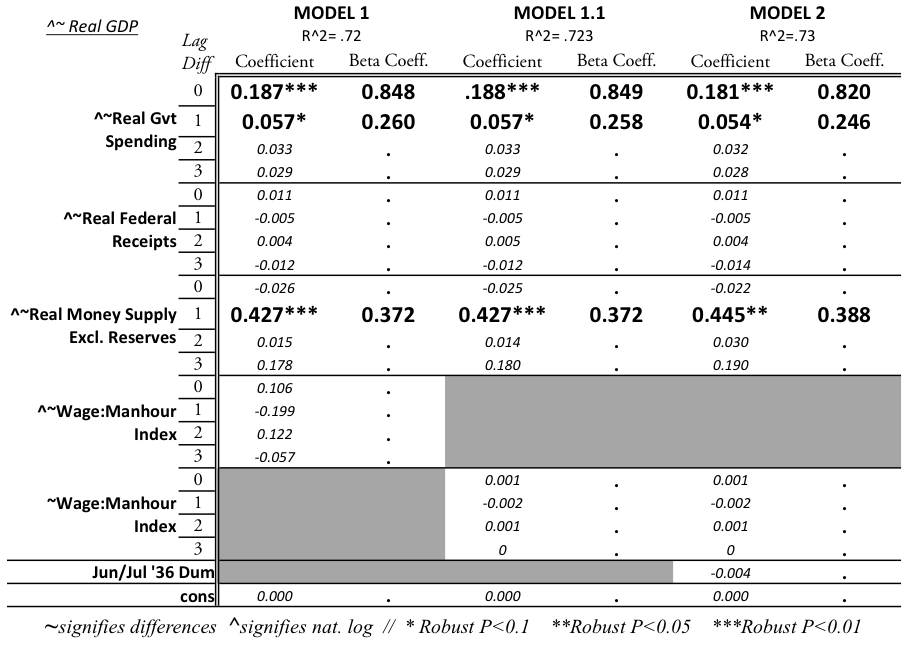
Table A-1
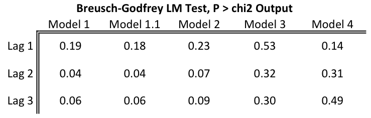
Table A-2
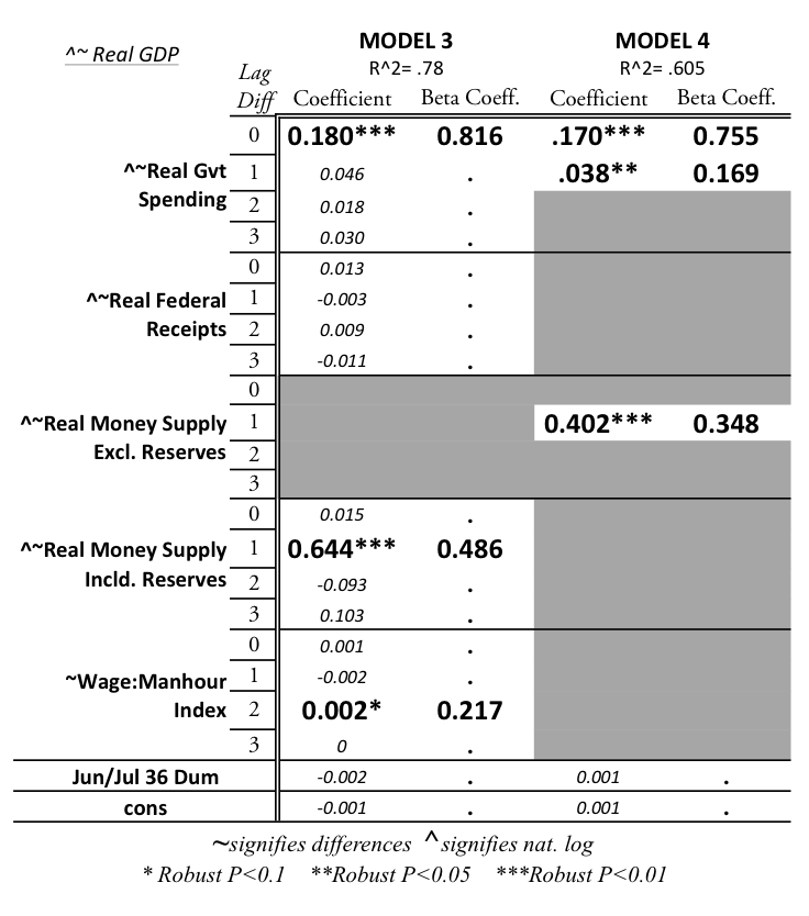
Table A-3
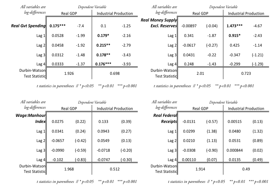
Table A-4. Simple regression of each independent variable on GDP or industrial production.
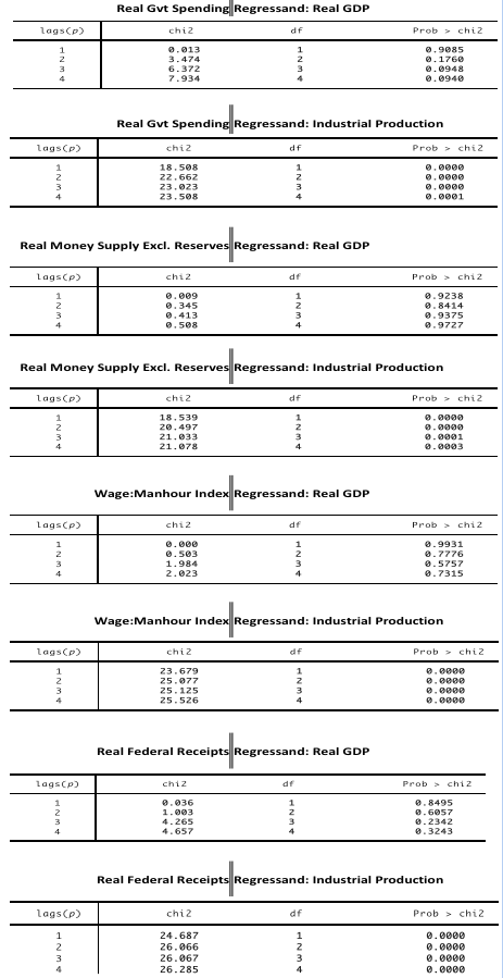
Table A-5. Breusch-Godfrey Test Results for Table A-4 regressions.
Figures
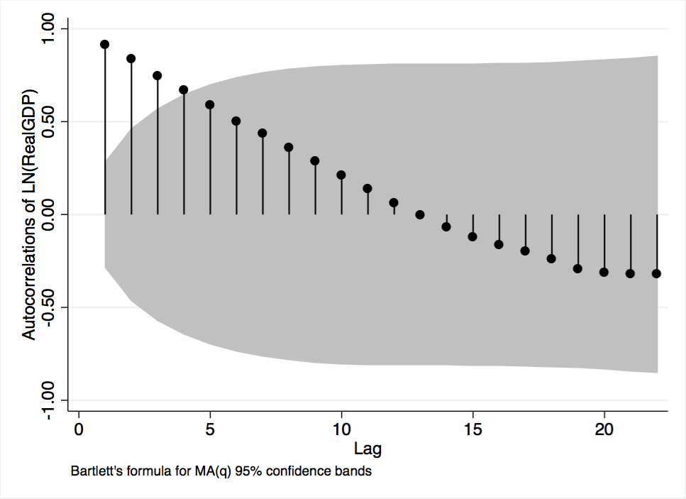
Figure A-1. Autocorrelation plot of GDP variable.
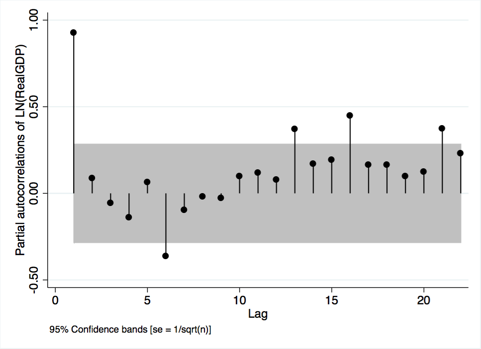
Figure A-2. Partial autocorrelation plot of GDP variable.
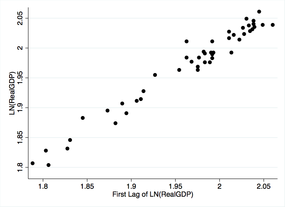
Figure A-3. Scatterplot of the GDP variable against its first lag.
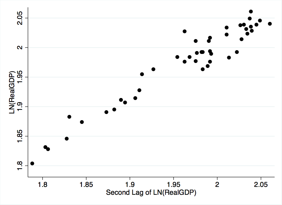
Figure A-4. Scatterplot of the GDP variable against its second lag.
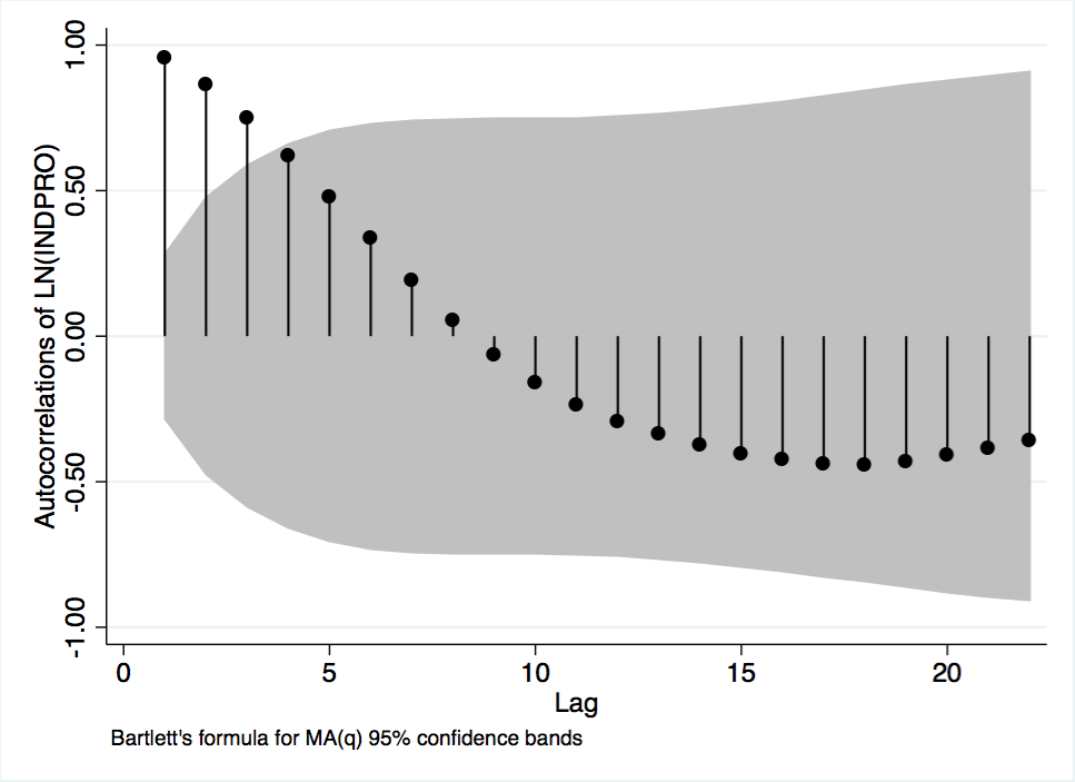
Figure A-5 Autocorrelations of Industrial Production
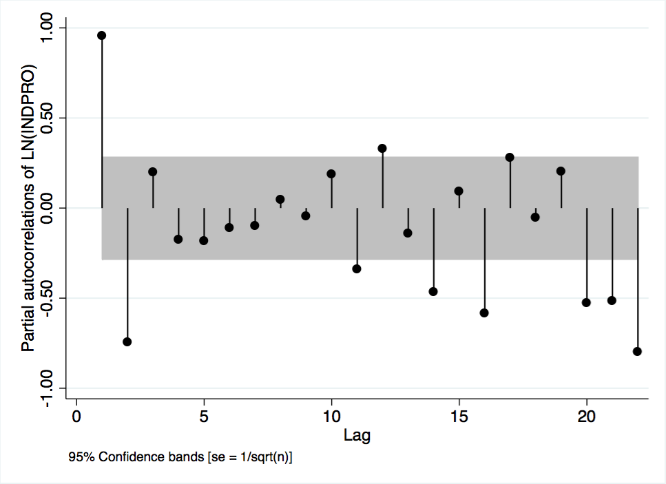
Figure A-6 Partial Autocorrelations of Industrial Production
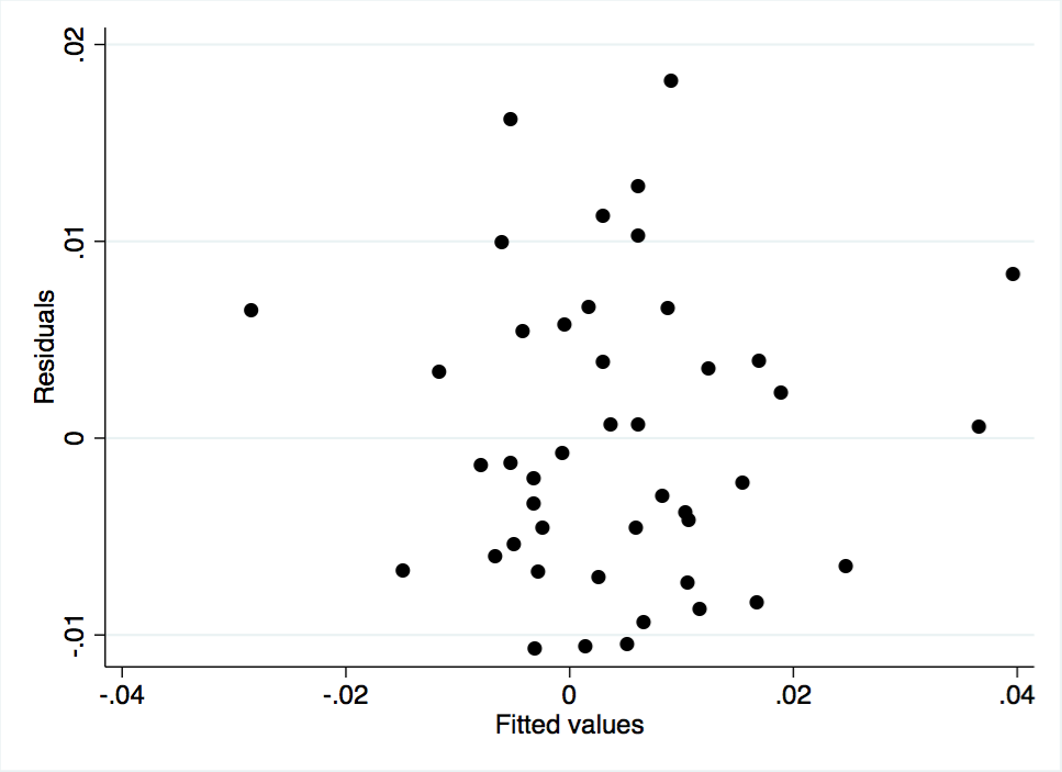
Figure A-7 Scatterplot of Model 1 Residuals Against Fitted Values
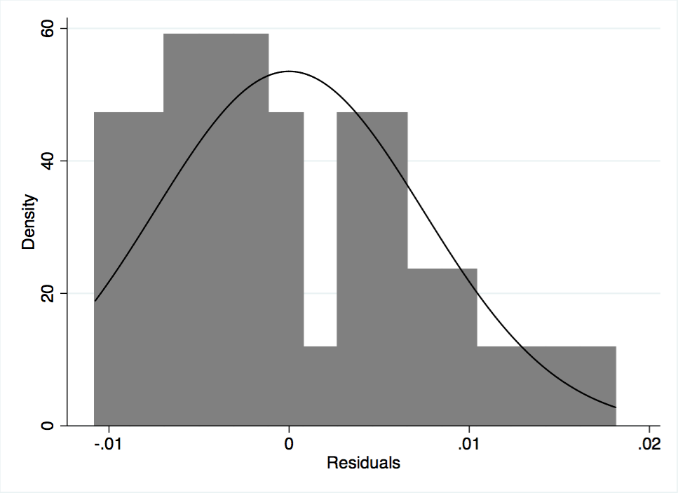
Figure A-8 Histogram of Model 1 Residuals
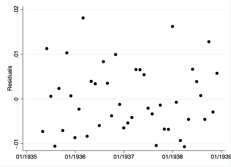
Figure A-9 Model 1 Residuals Plotted Over Time
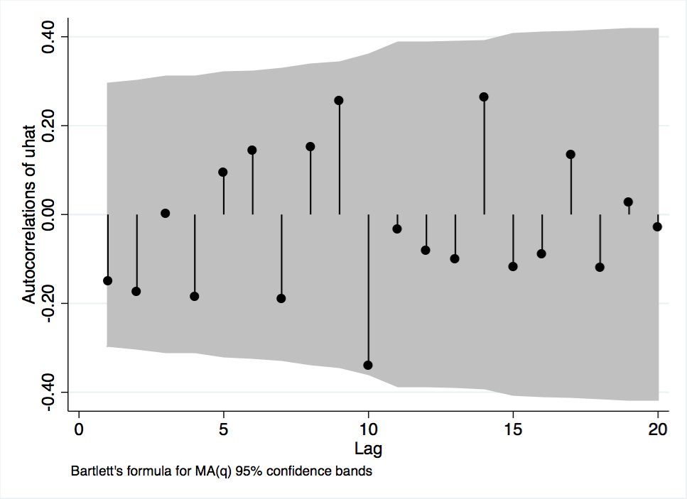
Figure A-10 Autocorrelations of Model 1 Residuals
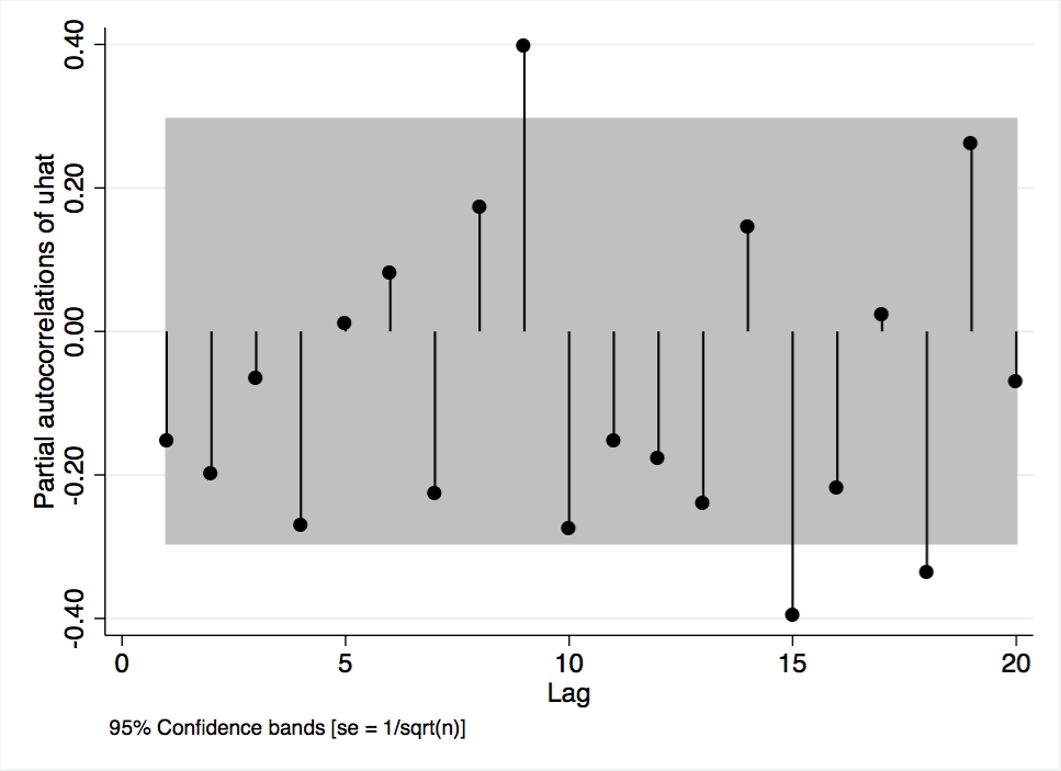
Figure A-11 Partial Autocorrelations of Model 1 Residuals
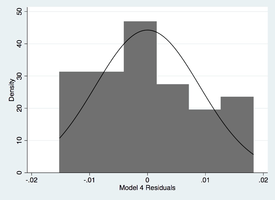
Figure A- 12. Histogram of Model 4 Residuals.
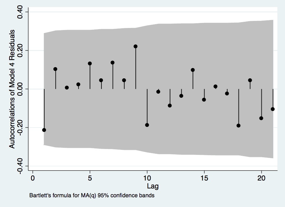
Figure A- 13. Autocorrelations of Model 4 Residuals.
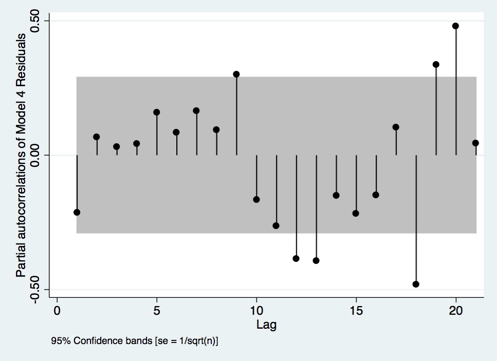
Figure A- 14. Partial Autocorrelations of Model 4 Residuals.
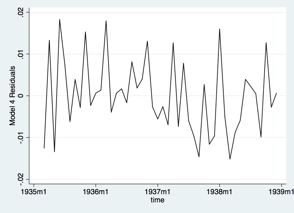
Figure A- 15. Lineplot of Model 4 Residuals.
Save Citation » (Works with EndNote, ProCite, & Reference Manager)
APA 6th
Rafti, J. (2015). "Roosevelt's Recession: A Historical and Econometric Examination of the Roots of the 1937 Recession." Inquiries Journal/Student Pulse, 7(06). Retrieved from http://www.inquiriesjournal.com/a?id=1053
MLA
Rafti, Jonian. "Roosevelt's Recession: A Historical and Econometric Examination of the Roots of the 1937 Recession." Inquiries Journal/Student Pulse 7.06 (2015). <http://www.inquiriesjournal.com/a?id=1053>
Chicago 16th
Rafti, Jonian. 2015. Roosevelt's Recession: A Historical and Econometric Examination of the Roots of the 1937 Recession. Inquiries Journal/Student Pulse 7 (06), http://www.inquiriesjournal.com/a?id=1053
Harvard
RAFTI, J. 2015. Roosevelt's Recession: A Historical and Econometric Examination of the Roots of the 1937 Recession. Inquiries Journal/Student Pulse [Online], 7. Available: http://www.inquiriesjournal.com/a?id=1053
Suggested Reading from Inquiries Journal
After years of economic downturn and recovery, the debate over stimulus packages and countercyclical policy continues globally. Proponents of such policies claim that the various stimulus packages and policy initiatives around the globe helped bring about quicker recovery, while opponents claim that in many cases these policies... MORE»
The Obama presidency will largely be defined by the administration’s ability to respond to the unique and historic challenge facing the country at the time of his inauguration: the Great Recession. This paper evaluates the president’s success throughout both of his terms in enacting an economic policy, which was largely... MORE»
The “Great Recession” of 2008 resulted in unprecedented levels of state deficit spending.[1] However, even though deficits are partly the result of economic forces beyond the control of state governments&mdash... MORE»
An exhibition entitled “The Quilts of Gee’s Bend” opened at the Whitney Museum of American Art in New York in November, 2002 (McGee), bringing worldwide attention to a secluded hamlet in a curve of the Alabama River. Unbeknownst to many of the admirers of these brightly patterned blankets was that the national spotlight had once before been shone on the town. That time... MORE»
Latest in Economics
2020, Vol. 12 No. 09
Recent work with the Economic Complexity Index (ECI) has shown that a country’s productive structure constrains its level of economic growth and income inequality. Building on previous research that identified an increasing gap between Latin... Read Article »
2018, Vol. 10 No. 10
The value proposition in the commercial setting is the functional relationship of quality and price. It is held to be a utility maximizing function of the relationship between buyer and seller. Its proponents assert that translation of the value... Read Article »
2018, Vol. 10 No. 03
Devastated by an economic collapse at the end of the 20th century, Japan’s economy entered a decade long period of stagnation. Now, Japan has found stable leadership, but attempts at new economic growth have fallen through. A combination of... Read Article »
2014, Vol. 6 No. 10
In July 2012, Spain's unemployment rate was above 20%, its stock market was at its lowest point in a decade, and the government was borrowing at a rate of 7.6%. With domestic demand depleted and no sign of recovery in sight, President Mariano Rajoy... Read Article »
2017, Vol. 9 No. 10
During the periods of the Agrarian Revolt and the 1920s, farmers were unhappy with the economic conditions in which they found themselves. Both periods witnessed the ascent of political movements that endeavored to aid farmers in their economic... Read Article »
2017, Vol. 7 No. 2
In 2009, Brazil was in the path to become a superpower. Immune to the economic crises of 2008, the country's economy benefitted from the commodity boom, achieving a growth rate of 7.5 per cent in 2010, when Rousseff was elected. A few years later... Read Article »
2012, Vol. 2 No. 1
The research completed aimed to show that the idea of fair trade, using the example of goals for the chocolate industry of the Ivory Coast, can be described as an example of the economic ideal which Karl Marx imagined. By comparing specific topics... Read Article »
|